Vector thinking for Max Profit

Occasionally I am lucky enough to run into a problem that doesn’t already have many vector solutions, so I can demonstrate how vector thinking can allow you to find an elegant solution. To build up to my insight let’s solve 2 easy variations and then we can get to the two more interesting puzzles.
The problem in question is called Best Time to Buy and Sell or more popularly simply Max Profit.
The theme is always the same you are given an ordered list of positive numbers that represent the evolution of the price of the security. You must find the maximum profit you could have made given this price series. You can only hold 1 unit at a time and you can not short, which means you must buy before you can sell (you can only profit from the price evolving upward).
The simplest and most well know variation is the 1 transaction problem (leetcode problem 121): you can only buy and sell at most 1 time what is the max profit that can be earned from the following series:
example series:
3 2 5 1 3 2 4 9 5 12 3 5
The key insight into this problem is that we are looking for the largest difference between the current element and the smallest element we have seen.
To motivate this insight, let’s look at ever larger versions of this problem starting with just one price to detect the pattern.
3 -> 0
Given just one price we can only buy and sell on the same day, so effectively max profit is 0
3 2 -> 0
Given these two points we can still only earn 0, since we must sell after we buy.
3 2 5 -> 3
Now that we have a higher number after a lower number we can plainly see that of the two options buy at 3 or buy at 2, buy at 2 and sell at 5 is better.
3 2 5 1 -> 3
The answer is still 3, since we can’t sell higher than 5, and even if we bought at 1 at the end there are no days left to sell
3 2 5 1 3 -> 3
We still do best by buying at 2 and selling at 5, buying at 1 and selling at 3 only earns 2.
3 2 5 1 3 2 -> 3
Plainly the 2 at the end doesn’t improve
3 2 5 1 3 2 4 -> 3
We can now either buy at 2 and sell at 5 or buy at 1 and sell at 4, but our max profit is still 3.
3 2 5 1 3 2 4 9 -> 8
Finally, the max profit changes! We can now buy at 1 and sell at 9. As new elements are added the new reward will be a function of the lowest element seen thus far.
We then get our solution:
{max x-mins x} 3 2 5 1 3 2 4 9 5 12 3 5
11, where we buy at 1 and sell at 12.
Or in python we could say something like:

import itertools
from operator import sub
def max_profit(p):
    return max(map(sub,p,itertools.accumulate(p,min)))

To unpack this a bit, mins returns the min element up to that point:
mins[3 2 5 1 3 2 4 9 5 12 3 5]
3 2 2 1 1 1 1 1 1 1 1 1
we can then do element-wise subtraction to see what the profit is from selling at each point
0 0 3 0 2 1 3 8 4 11 2 4
taking the running max we get the max profit so far,
0 0 3 3 3 3 3 8 8 11 11 11
we can see that this series is exactly the results that we got when we were looking at the max profit for the prefixes of the series.

Easy enough, let’s look at version 2 of this problem (leetcode 122):
unlimited number of transactions: We are now allowed to buy and sell as often as we like provided we never own more than 1 share of the stock and we still must sell after we bought. To make things easier we can assume that we can buy and sell on the same day, in practice this doesn’t matter as any day we do this we can consider that we did nothing.
Keeping the same price series as before:
3 2 5 1 3 2 4 9 5 12 3 5
We now notice that we should take advantage of every single time the price goes up. Again let’s look at a smaller example to get some intuition.
3 2 5 -> 3
Nothing fancy here, we buy at 2 and sell at 5, purchasing at 3 doesn’t improve our profit since selling at 2 would incur a loss.
3 2 5 1 3 -> 5
buy at 2 sell at 5, buy at 1 sell at 3
3 2 5 1 3 2 4 -> 7
just add one more purchase at 2 and sell at 4,
3 2 5 1 3 2 4 9 -> 12
Here it becomes interesting, we can look at two interpretations
buy at 2 sell at 5 (3),buy at 1 sell at 3 (2), buy 2 sell at 9 (7) for a total of 12
or we can say:
buy at 2 sell at 5 (3),buy at 1 sell at 3 (2), buy at 2 sell at 4 (2),buy at 4 sell at 9 (5) for a total of 12.
The two approaches are identical since addition commutes, it doesn’t matter how you get from 2 – 9 you will always earn 7.
Which means that we can simply add up the positive steps in the price series. That will be the maximum profit for an unlimited number of transactions:
Our code is simply:
{(x>0) wsum x:1 _ deltas x} 3 2 5 1 3 2 4 9 5 12 3 5
21
Deltas gives us the adjacent differences. We drop the first delta since we cannot sell before we have bought. If the delta is positive >0 we want to include it in our sum. Using (w)eighted(sum) we weight the >0 with a 1 and less then 0 or =0 are given a weight of 0.

Now that we covered the case with 1 transaction and unlimited transactions, we should feel confident that we can tackle 2 transactions. Lucky for us, that’s exactly version III of the problem (leetcode 123):
Getting insight into how to solve this variation should start with thinking about how we could solve this naively. The correct heuristic to reach for is divide and conquer. Suppose that for every step along the price evolution we knew what the max profit was before and the max profit was after. Then we could sum those two max profits and take the largest combination.

assume max_profit function as before:

r=range(len(p))
max([max_profit(p[0:i])+max_profit(p[i:]) for i in r)])

For our example this gives us 15.

What we might notice is that we are recomputing the max profit over for larger and larger prefixes, and for smaller and smaller suffixes.
We know that the prefixes were already computed simply by taking the rolling max instead of the overall max in max_profit. The only thing we’re missing is how to calculate the max_profit of suffixes.
Now we notice a symmetry – while the prefixes are governed by the rolling minimum, the suffixes are bounded by the rolling maximum from the left, i.e. the largest element available at the end to sell into.

To get a sense of this, look at the solutions to the suffixes
3 5 -> 2 (buy at 3 sell at 5)
12 3 5 -> 2 (buy at 3 sell at 5)
5 12 3 5 -> 7 (buy at 5 sell at 12)
9 5 12 3 5 -> 7 (buy at 5 sell at 12)
4 9 5 12 3 5 -> 8 (buy at 4 sell at 12)
Which leads to this solution in q:

{max reverse[maxs maxs[x]-x:reverse x]+maxs x-mins x}

maxs x -mins x / is familiar from earlier
If we want to walk backwards through a list, we can reverse the list and apply the logic forwards then reverse the result, which is the same as applying the logic to the suffixes.
So all we need to do is to subtract each element from the running maximum then take the running max of this result to get the max profit for the suffix so far.
In Python this simply becomes:

from itertools import accumulate as acc
from operator import add,sub
def max_profit_2trans(p):
    before=list(acc(map(sub,p,acc( p,min)),max))
    p.reverse()
    after=list(acc(map(sub,acc(p,max),p),max))
    after.reverse()
return max(map(add,b,a))

Alright, finally we should be able to tackle the most general version of this problem (leetcode 188). You are given both a series of prices and allowed to make up to k transactions. Obviously, if k is 1, we solved that first. We just solved k is 2. You can verify for yourself, but if k is larger than half the length of the price series the max is the same as the second problem we solved. Since every pair of days can allow for at most one transaction, effectively k is unlimited at that point.
We need to solve the k>2 but less than k<n/2. The standard CS technique that comes to mind is some kind of dynamic programming approach. To quote MIT’s Erik Demaine CS6006 dynamic programing is recursion plus memoization.
Let’s setup the recursive solution and assume we are at a particular (i)ndex in our price series, with k transactions left.
Let’s start with the base cases:
If k equals 0 we return 0
If i is greater than the last index, i.e. there are no elements left in the list: we return 0.
Otherwise the solution to the problem is simply the maximum of 2 options:

do nothing at this step:

0+the function increment i

do something:

If we are (h)olding a share we can sell at this step which adds the current price +the result of this function with one less k and i incremented by 1.
Otherwise we buy at this step, which is minus the current price (we spend money to buy) plus the result of this function with i incremented and we are now holding a share.

Here is the code for this in q:


p:3 2 5 1 3 2 4 9 5 12 3 5
cache:(0b,'0,'til[count p])!count[p]#0
f:{[h;k;i]$[i=count p;0;(h;k;i) in key cache;cache[(h;k;i)];
:cache[(h;k;i)]:.z.s[h;k;i+1]|$[h;p[i]+.z.s[0b;k-1;i+1];.z.s[1b;k;i+1]-p i]]}

We can test this and see that it results in the right answer for k=0,1,2
f[0b;0;0] -> 0 no surprise with 0 transaction no profit is possible
f[0b;1;0] -> 11 the original problem
f[0b;2;0] -> 15 buy at 1, sell at 9, buy at 5 sell at 12

However, we know that a vector solution is possible for k=1,2,infinity, so we might hope there is a vector solution for when k is 3 and above.
We can analyze the intermediate results of the cache to get some sense of this.

code to look at the table

t:(flip `h`k`j!flip key cache)!([]v:value cache)
exec (`$string[j])!v by k from t where not h 

output table:

 | 11 10 9 8 7 6  5  4  3  2  1  0 
-| --------------------------------
0| 0  0  0 0 0 0  0  0  0  0  0  0 
1| 0  2  2 7 7 8  10 10 11 11 11 11
2| 0  2  2 9 9 12 14 14 15 15 15 15
3| 0  2  2 9 9 14 16 16 17 17 18 18
4| 0  2  2 9 9 14 16 16 18 18 20 20

What we might notice is that the first row is the running maximum from selling at the prefixes. Then it’s the combination of the previous row and 1 additional transaction. In other words, each row allows you to spend money from the previous row and sell at the current price.
Putting this into action we get the following:

{[k;p]last {maxs x+maxs y-x}[p]/[k;p*0]}

We can look at intermediate rows by writing the scan version of the code and we know it will converge to the unlimited transaction case:

{[p]{maxs x+maxs y-x}[p]\[p*0]} p
0 0 0 0 0 0 0 0  0  0  0  0 
0 0 3 3 3 3 3 8  8  11 11 11
0 0 3 3 5 5 6 11 11 15 15 15
0 0 3 3 5 5 7 12 12 18 18 18
0 0 3 3 5 5 7 12 12 19 19 20
0 0 3 3 5 5 7 12 12 19 19 21

What’s really nice about this code is that it actually describes the problem quite well to the computer and in effect finds exactly what we want.
p*0 / assume we have 0 transactions and therefore 0 dollars at each step.
y-x / subtract the current price(x) from the current profit(y) element wise
maxs y-x/ find the rolling max revenue
x+maxs y-x / add back the current selling price
maxs x + maxs y-x / find the rolling max profit
repeating this k times finds the max profit of the k’th transaction.

Here is the python code that implements this logic:

import itertools
from operator import add,sub
def max_profit(k: int, prices: List[int]) -> int:
        if k==0 or len(prices)<2:
            return 0
        z=[0]*len(prices)
        maxs=lambda x: itertools.accumulate(x,max)
        addeach=lambda x,y: map(add,x,y)
        subeach=lambda x,y: map(sub,x,y)    
        for i in range(k):
            z=maxs(addeach(prices,maxs(subeach(z,prices))))
        return list(z)[-1]

I think this post covers this puzzle, let me know if there are interesting variations I haven’t explored.
Advertisement

Idempotent + Moving Window is simply a reduction

I want to calculate the moving window max or min in a data parallel way.
Lets start with the two argument function max

max(x,y) returns the greater of x and y
max(x,x) returns x (idempotent)

max(5,3) return 5

max(max(5,3),max(5,3)) reduces to max(5,5) which just returns 5

If we want max of an entire list we can simply think of it as a reduction in the lisp/APL sense

max(head (x), (max (head (tail (x), max( head(tail(tail(x))), …. )

or in a more readable way, replace max with |, and insert it between every element in the list

x[0] | x[1] | x[2] | x[3] this is a standard reduction/over.

Here is a concrete example:

x:5 4 3 2 7 2 9 1

Max over(x) –> 9

|/x –> 9

We can look at the intermediate results

Max scan(x) –> 5 5 5 5 7 7 9 9

|\x –> 5 5 5 5 7 7 9 9

Now let’s say that we want to look at the 3 slice moving window.

Let’s take advantage of the fact that max(x,x) yields x, idempotent

We can calculate the max between each pair in our list. Read max each-prior (‘:)

(|’:)x –> 5 5 4 3 7 7 9 9

applying this function n-1 times gives us a moving max

so (|’:) (|’:) x is 3 slice moving window, which we can rewrite as
2 |’:/ x

5 5 5 4 7 7 9 9

We can see that |\x is equivalent to (count[x]-1) |’:/ x which is data parallel by construction. In other words, we are doing an adjacent transform.

To make this a bit clearer, we can show intermediate results by using a scan(\) instead of an over(/)

(count[x]-1)|’:\x

5 4 3 2 7 2 9 1
5 5 4 3 7 7 9 9
5 5 5 4 7 7 9 9
5 5 5 5 7 7 9 9
5 5 5 5 7 7 9 9
5 5 5 5 7 7 9 9
5 5 5 5 7 7 9 9
5 5 5 5 7 7 9 9

One thing we can notice is that we could terminate early, since we know that if an adjacent element did not change there is no way for the max value to propagate further.

Which means we can rewrite (count[x]-1)|’:\x to simply (|’:\)x

and indeed this gives us:

(|’:\)x

5 4 3 2 7 2 9 1
5 5 4 3 7 7 9 9
5 5 5 4 7 7 9 9
5 5 5 5 7 7 9 9

Technically this is still slower than maxs(x) but if we had gpu support for each-prior(‘:) we could calculate maxs in n calls to max prior which has a parallelization factor of n/2. Depending on the range of x, the n calls might be bound significantly such that for small ranges, for example you are dealing with a short int (8 bytes), you can effectively compute the maxs in O(c*n/2) time with parallelism. Where c is a function of the effective range of your inputs — max[x]-min[x].

Now let’s get back to the problem of max in a sliding window, like this leetcode problem. This problem is classified as hard and the reason is that leetcode doesn’t want you to use parallelism to solve sliding window, it wants you to do it in O(n) time directly.

We know we can solve the problem in O(n) time when the window is equal to 1,2, and n.
identity({x}), max each prior ({|’:x}), and maxs ({|\x}) respectively.

The key to solving it for all window sizes is to recognize that each entry only depends on itself and its neighbors and that the result is the same if you duplicate neighbors – again idempotentcy comes to the rescue. max(1 2 3) is equal to max(1 1 2 2 3 3). Another good explanation can be found here. This is technically a dynamic programming approach with two pointers, but I have never seen it explained in what I think is the most straightforward way.
Let’s borrow the example from leetcode and work through what should happen.

Suppose list of numbers n=1 4 3 0 5 2 6 7 and window size k=3. Then reusing the prior code to show intermediate steps, we get:

1 4 3 0 5 2 6 7
1 4 4 3 5 5 6 7
1 4 4 4 5 5 6 7

If we look at a particular slot, 0 for example, it gets overtaken by 4, but the 5 slot only needs to compete with 3. In other words, each element is looking at at most n-1 elements to the right and n-1 elements to the left. So we can rearrange n to do this in a natural way. Let’s reshape n, so that there are k columns. q supports ragged arrays, so our last row is not the same length which is nice.

q)(0N;k)#n
1 4 3
0 5 2
6 7

We can then compute the maxs of each row

q)maxs each (0N;k)#n
1 4 4
0 5 5
6 7

And flatten it back:

q)l:raze maxs each (0N;k)#n
q)l
1 4 4 0 5 5 6 7

This gives us our left window. Now we will repeat the steps but instead of going from the left we will go from the right.
The simplest way go from the right is to reverse the list apply the function as normal from the left and reverse the list again. In J this operation is called under, as in going under anesthesia, perform the operation and then wake you from the anesthesia. This is equivalent to looking at the cummulative max from the right or walking backward through the array.

q)under:{[f;g](f g f ::)}
q)(reverse maxs reverse)~under[reverse;maxs] /this is the same
1b 

q)(reverse maxs reverse ::) each (0N;k)#n
4 4 3
5 5 2
7 7

Now we just need to flatten the list and call it r.

q)r:raze (reverse maxs reverse ::) each (0N;k)#n

Because r is going from the right, we need to shift it by k-1 elements to the right so that we are not using data from the future when looking at what the current max should be. Printing l on top of r, we get:

q)(l;(k-1) xprev r)
1 4 4 0 5 5 6 7
0N 0N 4 4 3 5 5 2

As we can see, a simple max along the columns will give us the correct answer. (Note: the 0N in the beginning correspond to nulls)

q)max (l;(k-1) xprev r)
1 4 4 4 5 5 6 7

This idea can be generalized, so let’s write a generic function that can take an idempotent operation and create a moving window version.

fmx:{[f;g;h;m;x]l:raze (f')w:(0N;m)#x;r:raze (g')w;h[l;(m-1) xprev r]}

fmx takes a function f that will be applied to generate the left window, a function g that will be used to generate the right window and h a function that will combine left and right windows shifting r based on the window.

We can now generate (mmax, mmin, mfill):
fmmax:fmx[maxs;(reverse maxs reverse ::);|]
fmmin:fmx[mins;(reverse mins reverse ::);{&[x;x^y]}] /fill the nulls with x
fmfill:fmx[fills;(reverse ({y^x}) reverse ::);{y^x}]

We can also generate a function that will allow us to inspect what elements we have access to in the right and left windows so that we can debug/make new functions, with some small modifications.

inspect:fmx[,\;(reverse (,\) reverse ::);{([]l:x;r:y)}]

Here we define f to concatenate the elements seen so far, g is the reverse concatenate, and h is return a table of the l and r.

When we run inspect on our original n, we see that every row has the information from the appropriate sliding window in it, though sometimes more than once.

q)inspect[k;n]
l      r       
--------------
,1     `long$()
1 4    `long$()
1 4 3  1 4 3   
,0     4 3     
0 5    3       
0 5 2  0 5 2   
,6     5 2     
6 7    2       

We can see that the combination of left and right windows will always have at least the three elements required.

To summarize, we saw that idempotent functions, like max and min, allow for parallelization and allow us to use the dynamic programming two pointer technique to solve sliding window calculation in O(n).


Below is the python code for sliding maximum window, written in numpy/APL style, I’m not sure it makes the concept clearer, but more people read python than q. numpy doesn’t like ragged arrays, so there is a bit of extra code to handle the cases where count of n is not evenly divisible by k.

def maxSlidingWindow(k,nums)
  cmax=np.maximum.accumulate
  n=len(nums)
  z=np.zeros(k*np.ceil(n/k).astype(int))
  z[:n]=nums
  z=z.reshape(-1,k)
  l=np.resize(cmax(z,1).reshape(z.size),n)
  r=np.resize(np.flip(cmax(np.flip(z,1),1),1).reshape(z.size),n)
  return list(np.max(np.stack([l[k-1:],r[:r.size-(k-1)]]),0).astype(int))

all code can be found here:
https://github.com/pindash/q_misc/blob/master/sliding_window_max.q

Stable Marriage in Q/KDB

A friend of mine is applying to Medical Residency programs, which motivated me to investigate the matching algorithm used to match residents with hospitals. NRMP the organization behind the matching process has a dedicated video explaining how the algorithm works. The simplest version of the problem can be thought to consist of n guys and n gals who are looking to pair off. Each gal has a ranked list of guys and each guy a ranked list of gals. We want to find a pairing such that no guy and gal can pair off and be better off. We call this stable, since any gal who wants to leave can’t find a guy who isn’t currently happier with someone else. It takes two to tango, or in this case disrupt a stable pairing.

Gale-Shapley published a result on this problem in 1962 showed a few amazing properties:

  1. A stable pairing always exists
  2. There is an algorithm to get to this pairing in O(n^2)
  3. It is truthful from the proposing side, i.e. if men are proposing then they can’t misrepresent their preferences and achieve a better match
  4. The proposing side gets the best stable solution and reviewing side gets the worst stable solution
  5. The reviewing side could misrepresent their preferences and achieve a better outcome

Knuth wrote about this problem pretty extensively in a French manuscript. The University of Glasgow has become a hub for this problem, Professor Emeritus Robert Irving wrote the book on the topic and his student David Manlove has written another. New variations and approaches keep coming out, so in a way this problem is still an active area of research. For this post I want to look at only the simplest version and describe a vectorized implementation.

First let’s walk through an example by hand (note: lowercase letters are men)

Men ranking women

d| `D`B`C
b| `B`C`D
c| `C`D`B

Women ranking men

D| `b`c`d
B| `b`c`d
C| `d`b`c

First we pair off d,D
Then we pair off b,B
Finally we pair c,C

If we had started from the women:

First we pair D,b
Then we pair B,b and drop D to be unpaired, because b prefers B to D
Then we pair D,c
Finally we pair C,D

So we see there are two stable pairings. B always pairs with b, but either the men (d,c) or the women (D,C) will get their worst choice.

The algorithm:

Propose a pairing and engage the pair:

  • If the reviewing party (woman) prefers the current proposing party to her current engagement:
    1. Jilt the current party (A jilted party goes back into the pile of unengaged proposing parties, with all the parties he has proposed to so far crossed off)
    2. Become engaged to the proposing party (A reviewing party always prefers any partner to being alone)
  • If the current proposal did not work:
    1. Continue down the ranked list of the proposing party until they find a match, i.e. go back to ste

Here is how we can implement the naive version of this algorithm in Q/KDB:

Here is how we can implement the naive version of this algorithm in Q/KDB:
i:3 /number of each party
c:0N /number of ranked individuals on each list 
     /(null takes a random permutation, convenient since we want everyone to rank everyone) we can also use neg[i]
m:neg[i]?`1 /choose i random symbols with 1 char to represent each possible man
w:upper m /assign same symbols but upper case as list of all possible women
dm:m!(#[i;c]?\:w) /create a dictionary of male preferences
       / each man chooses a random permutation of women
dw:w!#[i;c]?\:m /each women chooses a random permutation of men
t:1!([]w:w;m:`;s:0W) /our initial pairing table, each women is unpaired, 
	          /so her current score is infinity, 
	          /the table is keyed on w, so that a women can only have 1 match
ifin:{$[count[x]>c:x?y;c;0W]} 
 /ifin returns the position in the list like find(?), 
 /but returns infinity if not found instead of length of list
 /example 
 /ifin[`a`b`c;`b] --> 1 
 /ifin[`a`b`c;`d] --> 0W 
The algorithm
f:{[t]
 if[null cm:first key[dm] except (0!t)`m;:t];
 im:first where t[([]w:k);`s]>s:dw[k:dm cm]iifin\: cm;
 t upsert (k im;cm;s im)};

f takes a pairing table of the current pairings. It then looks for the first unmatched man. We call this (c)urrent (m)an, if current man is null, we are done all men are matched, return t, our pairings.

Otherwise, find the first woman on his list of ordered rankings whose happiness (s)core he can improve. We are using iifin to see where his rankings score from the women’s side, and by choosing the first such match, we are preferencing his choice. We then insert this pair into the pairing (t)able, along with the happiness (s)core.
f over t /repeat the process of adding pairs into the table until all men are matched.

Before we look at the vectorized (batched) version, there are some simple optimizations we can make. For example, since we notice that we will be calculating how much a woman likes a man back when he chooses her, we can pre-tabulate all pairs in advance.

Here is the code that creates a table that will have every man and woman pairing with both his and her score next to it:

/first convert the dictionary to a table that has each man and his rankings
/along with a column which ranks the match, 
tm:{([]m:key x;w:value x;rm:(til count ::)each value x)} dm
/looks like 
m w     rm   
-------------
m E M P 0 1 2
e P M E 0 1 2
p M E P 0 1 2
/then ungroup looks like this:
tm:ungroup tm 

m w rm
------
m E 0 
m M 1 
m P 2 
e P 0 
e M 1 
e E 2 
p M 0 
p E 1 
p P 2 

repeat the procedure with women's table. 

tw:ungroup {([]w:key x; m:value x;rw:(til count ::) each value x)} dw

/now left join each match 
ps:tm lj `w`m xkey tw
m w rm rw
---------
m E 0  2 
m M 1  0 
m P 2  1 
e P 0  2 
e M 1  2 
e E 2  1 
p M 0  1 
p E 1  0 
p P 2  0 

Now that we have pre-computed all the scores we can look at the vectorized version:

First, we notice that we can technically make proposals from all the men in one batch. There is one caveat, if two or more men rank one woman as their top choice during a matching batch the tie is broken by the woman. So we can grab each man’s current first choice and break all the ties with that woman’s ranking.

Second, we notice that any woman who is currently engaged will stay engaged unless a man she desires more becomes available. This means we can eliminate all women who are already engaged to someone they prefer more from each man’s ranking. In other words, if Alice is currently engaged to Bob, and she prefers only Carl to Bob, Sam doesn’t stand a chance and we can eliminate Alice from Sam’s ranking completely.

These two tricks are all it takes to vectorize(batch) the solution.

Now let’s look at the code:

Here is the algorithim in one block:

imin:{x?min x} /get the index of min element
smVec:{[ps;t]ms:exec last s by w from t;
 update check:(check+1)|min rm by m from ps where not m in (0!t)`m,rw<ms[w];
 p:select m:m imin rw, s:min rw by w from ps where rm=check;t upsert p}

Let’s break it down statement by statement:

smVec:{[ps;t]
/
/ smVec takes a data table which are our (p)recomputed (s)tatistics 
/ it also takes the pairs table t, which is the same as above
/
 ms:exec last s by w from t;
/
/ms is our current best score for each woman who is currently engaged
/
 update check:(check+1)|min rm by m from ps where not m in (0!t)`m,rw<ms[w];
/ For each man we keep a counter of who we should check next, 
/ we increment this each time he is not yet engaged (not m in (0!t)`m) 
/ so we look at his next viable candidate, 
/ also we remove any candidates that he cannot satisfy (rw<ms[w]). 
/ He needs a woman who prefers him to her current match.
/ So we take the max of either the next candidate 
/ or the next one whose score would go up if he matched.
 p:select m:m imin rw, s:min rw by w from ps where rm=check;
/ now we simply select all the ones to check and break ties by min rw,
/ ie the woman's rank.
 t upsert p}
/lastly update/insert current matches into the pairings table

We need a stopping condition so that we can stop iterating:

Originally, I thought we need a condition that said something like “as long as there are unmatched men, keep iterating. {not all key[dm] in (0!x)`m}”

pairings:smVec[update check:-1 from ps]/[{not all key[dm] in (0!x)m};t]

As it turns out, once we remove all the clutter and always append only viable matches this turns out to be unnecessary. We can simply iterate until convergence which is the default behavior of over(/). So running the function looks like this:

pairings:smVec[update check:-1 from `ps] over t

We are done, but we can extend this one step further by allowing for incomplete preference rankings. The canonical way to treat incomplete ranking is to assume that a person would rather be a widower than be married to someone he didn’t rank.


To do this, we simply add the person matching with himself at the end of every ranking and add a shadow woman which is just the man ranking himself first. This means that once we get to the end of his ranked list he will automatically match with himself. With this small addition to the data, the complete setup function looks like this:

setup:{[i;c]c:neg c;m:neg[i]?`4;w:upper m;
 dm:m!(#[i;c]?\:w),'m;dw:w!#[i;c]?\:m;
 dw,:(m!0N 1#m);t:1!([]w:w,m;m:`;s:0W);
 tm:{([]m:key x;w:value x;rm:(til count ::)each value x)} dm;
 tw:{([]w:key x; m:value x;rw:(til count ::) each value x)} dw;
 ps:ej[`m`w;ungroup tm;ungroup tw];
 `dm`dw`t`ps set' (dm;dw;t;ps)}
setup[1000;0N] /ON means rank every member. 
pairings:smVec[update check:-1 from `ps] over t

Now we can verify that we have the right solution by comparing to the official python implementation

/write out some test data for python
setup[1000;0N]
pairings:smVec[update check:-1 from `ps] over t
`:m.csv 0: "," 0: ungroup {([]m:key x;w:-1 _' value x)}dm
`:w.csv 0: "," 0: ungroup {([]w:key x;m:value x)}count[dm]#dw

/python solve: (we need to increase the recursion limit in python because the library can't solve large problems without it, also I wasn't able to run problems bigger than 2000 on my machine without a segfault)
/
import pandas as pd
from matching.games import StableMarriage
import sys
sys.setrecursionlimit(50000)  
m=pd.read_csv("m.csv") 
w=pd.read_csv("w.csv") 
md=m.groupby("m")['w'].apply(list).to_dict()  
wd=w.groupby("w")['m'].apply(list).to_dict()  
game=StableMarriage.create_from_dictionaries(md,wd)
s=game.solve()
pd.DataFrame([(k, v) for k, v in s.items()], columns=["m","w"]).to_csv("mwsol.csv", index=False)

\
pysol:("SS";enlist ",") 0: `mwsol.csv
pysol:pysol lj update mm:m from pairings
0=count select from pysol where mm<>m

If we join on the women and our men match the python men, then we have the same answer.

Lastly, a note on performance: we get a 3x performance boost from vectorization
The naive version solves the
\t pairs:f over t
5000 -> 185771 (3 min)
2000 -> 15352 (15 sec)
1000 -> 2569 (2.5 sec)
\t smVec[update check:-1 from `ps] over t
5000 -> 59580 (1 min)
2000 -> 4748 (5 sec)
1000 -> 1033 (1 sec)

The python version takes 20 seconds when n is 1000 and I couldn’t test higher.
Which is about 7x slower than naive in q, and 20x slower than vectorized.

Further the python library doesn’t allow for incomplete preference lists. (we can create complete lists that have sentinels values where the list ends, but the memory usage is prohibitively expensive for large problems). Lastly, the python library runs into the recursion limit, which we avoided by iterating over a state data structure instead of using the stack.

Meanwhile in practice there are about 40k med students a year and each only ranks less than 100 choices. Which means we can solve that problem really quickly.
setup[100000;100]
\t pairings:smVec[update check:-1 from `ps] over t
1465 (1.5 seconds)

In the next post, I will describe how to extend this solution to apply the stable marriage problem to resident hospital matching problem where each hospital may have more than 1 slot.

Fifo Allocation in KDB

One of the most common questions in trading is how to attribute profits and losses. There are many ways of doing this each have their own advantages one of the simplest is first in first out allocation. Here is the basic concept illustrated with an example, I buy 7 apples for 10 dollars, sell 4 for 11 dollars, buy 2 more for 12 and sell 3 for 11 and then sell 2 more for 12. We can think of having a list of purchases 7,2 and list of sales 4,3,2. Each sale and purchase are associated with a price. No matter the allocation strategy, we know the profit can be calculated by a weighted sum of the sales ((4*11)+(3*11)+(2*12)) minus a weighted sum of the purchases ((7*10)+(2*12)) –> 7 dollars. Allocation tries to answer the question of which trades were bad. First in first out will allocate the first 7 sales to the first 7 purchases (7 dollars profit), leaving 2 more purchased and 2 more sold and allocate those to each other (0 profit). This tells us that all the profit was made from the first 7 purchased. However, a last in first out strategy might instead see this ((4*11)-(4*10)+((2*11)-(2*12))+((1*11)-(1*10))+((2*12)-(2*10)) which suggests that the second purchase at 12 dollars was a bad trade.

We leave the discussion for more elaborate allocation methods and their respective merits for another time. In this post we will focus on the mechanics of efficiently calculating fifo allocations. Luckily, Jeff Borror covers an elegant implementation in Q for Mortals, which I will only briefly repeat here. The idea is that you can represent the buys and sells as a matrix, where each cell corresponds to the amount allocated to that purchase and sale. By convention rows will correspond to purchases and columns to sales. So in our example, we can write the allocation as

 | 4 3 2
-| -----
7| 4 3 0
2| 0 0 2

I left the corresponding order quantities in the row and columns as headers but they are actually implied. Jeff also gives us the algorithm that produces this matrix.

  • First we calculate the rolling sums of the purchase and sales
    • 7 9 for purchases
    • 4 7 9 for sales
  • We then take the cross product minimum
    • 4 7 7
      4 7 9
  • We then take the differences along the columns
    • 4 7 7
      0 0 2
  • We then take the differences along the rows
    • 4 3 0
      0 0 2
  • We are done, as a bonus here is the code in Q
    • deltas each deltas sums[buys] &\: sums[sells]

Not only is this rather clever, there is a certain logic that explains how to come to this result. The cumulative sums tells you how much max inventory you have bought or sold till this point. The minimum tells you how much you can allocate so far assuming you haven’t allocated anything. The differences down the columns subtracts the amount you have already allocated to the previous sales. The differences along the rows tells you how much you have already allocated to the previous purchases. Since you can only allocate what hasn’t yet been claimed.

Having read this far, you should feel confident you can easily do fifo allocations in KDB. I know, I did. There are even stack overflow answers that use this method. There is one problem, that occurs the moment you start dealing with a non trivial number of orders. This method uses up n^2 space. We are building a cross product of all the buys and sells. We know that the final matrix will contain mostly zeros, so we should be able to do better. We can use the traditional method for doing fifo allocation. Keep two lists of buys and sells allocated thus far and keep amending the first non zero element of each list and created a list of allocations triplets, (buy, sell, allocated). Although, this is linear implementing this in KDB is rather unKdb like. For incidental reasons, amending data structures repeatedly which is what this algorithm entails is best done by pointers, which in KDB means using globals and pass by reference semantics. It’s not long, but it’s not pretty.

codecomment
fastFifo:{[o]/takes orders signed to neg are sell
signed:abs (o unindex:group signum o);/split into buys and sells
if[any 0=count each signed 1 -1;:([]row:();col:();val:())];/exit early if there are no buys or no sells
k:(/Brains of the calculation called k (for allokate)
.[{[a;i;b;s]/args are allocations triplets(a), index(i), buys(b), sells(s)
if[0=last[get s]&last[get b];:(a;i;b;s)];/if either there are no more buys or sells to allocate, return the current allocations
l:a[;i];l[2]:$[c:b[l 0]<=s[l 1];b[l 0];s[l 1]];/l is the current allocation, if (condition c) is buys are bigger allocate the sell qty, otherwise the buy qty
(.[a;(til 3;i);:;l+(0 1 0;1 0 0)c];i+:1;@[b;l 0;-;l 2];@[s;l 1;-;l 2])}]/depedning on the c increment either buy or sell pointer
);/end definition of k
`.fifo.A set (3;count[o])#0;/create global list of allocation triplets, size of total orders is at least 1 more than max necessary size, consider a case where you have 10 sells for 1 qty, 1 buy for 10, you will have 9 allocations
`.fifo.B set signed 1;/Set the buys
`.fifo.S set signed -1;/Set the sells
res:{delete from x where 0=0^val} update row:unindex[1] row, col:unindex[-1] col, next val from flip `row`col`val!get first k over (`.fifo.A;0;`.fifo.B;`.fifo.S);/delete the cases of 0 allocation, return the original indexes of the orders after apply k until the allocations stop changing, return the allocations as a sparse representation of the matrix
delete A,B,S from `.fifo;/delete the global variables to clean up
res}/return the result

This algorithm, has sufficient performance that we could stop there. However, we could ask is there a way to get all the benefits of the elegant array solution without paying the space cost. The answer is that we can, the trick is that as we have noticed most of the matrix will actually be filled with zeros. In particular, we can see that the matrix will essentially traverse from the top left hand corner to the bottom left hand corner. If we could split the problem into small pieces and then stitch the solutions together we would have the original path of allocations.

I will now briefly sketch out how we can split this problem into pieces and then I will present an annotated version of the code.

If we just look at the first 100 buys and first 100 sells. We can simply apply Jeff’s algorithm. If we wanted to apply it to the next 100 buys and next 100 sells, we would find that we have a problem. We need to know three things, we need to know the index of the buys and sells we are currently up to and any remaining buys and sells that we have not allocated to yet in the previous iteration. Strictly speaking we can only have unallocated quantities on one side, but it is easier to simply keep track of both and letting one list be empty each time.

Here is the annotated code:

codecomment
fifoIterative2:{[o]/takes orders signed, neg are sell
signed:abs o unindex:group signum o;/split into buys and sells
iterate:{[a;b;s]/Brains of the calculation called iterate takes accumulator (a), chunks of (b), chunk of sells (s), accumulator has three slots, slot 0 is for the current count where we are up to in the buys and sells, slot 1 keeps track of the unallocated qty from the previous iteration, slot 3 keeps track of the currrent allocations
if[any 0=sum each (b:a[1;`b],:b;s:a[1;`s],:s);:a];/concatenate the unallocated qty to the respective places and check if one is an empty list, if so exit early and return the accumulator
t:sm m:deltas each deltas sums[b]&\:sums s;/apply Jeff’s algorithm and shrink matrix to sparse rep
c:(sum .[0^m;] ::) each 2 2#(::),i:last[t][`col`row];/Sum the last col, and last row allocated so that we can calculate the amount allocated to the last buy and sell respectively
a[1]:`s`b!.[i _’ (s;b);(::;0);-;c];/drop all the buys and sells that were fully allocated and subtract the amount allocated on the last buy and sell, from the first of what’s left assign this to slot 1, which holds the remainder
a[2],:update row+a[0;`b], col+a[0;`s] from t;/Append to slot 2 the current allocations, updating the indexes using the counts from slot 0
a[0]+:(`s`b!(count[s];count[b]))-count each a[1];/update the count, adding to the count the currently allocated and subtracing the remainder
a};/return a
k:max div[;200] count each signed;/calculate the max  number of rows so that each buys and sells has at most 200 elements, configurable to the maximize efficiency of the machine
res:last iterate/[(`s`b!(0;0);`s`b!(();());sm 1 1#0);(k;0N)#signed 1;(k;0N)#signed -1];/reshape the buys and sells and iterate over the chunks, select the last element which is the allocations
update row:unindex[1]row,col:unindex[-1] col from res}/reindex the buys and sells into the original indexes provided by the input o

This code actually performs much faster than the iterative version and is shorter. This code essentially has no branching except where there are no more allocations on one side and exits early.

If anyone has a better way of computing fifo allocation let me know in the comments.

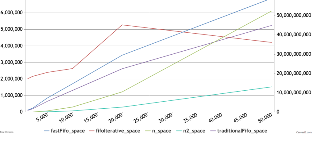
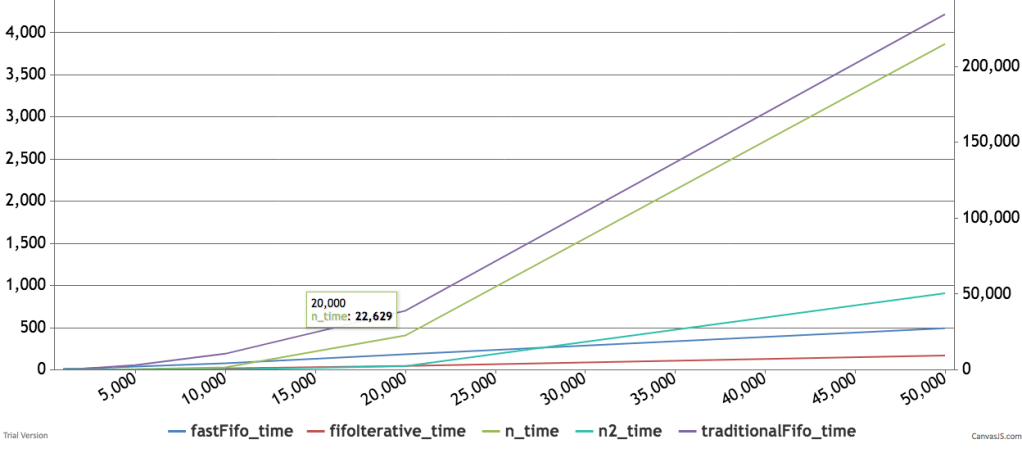
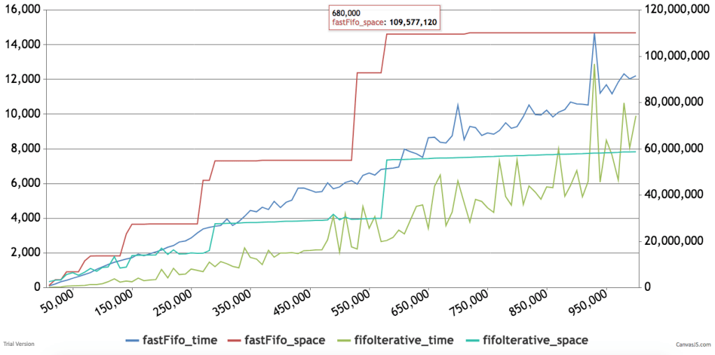
Below are some timings and graphs of memory usage. The code can be found here.