Every home cook knows that to get that extra dose of flavor, one needs to toast their spices like all the professionals. I’m here to tell you this not only unnecessary it’s counter productive.
The stated reason for this practice is that it release the aromatics makes the spices that much more potent. If you stop to consider this, it’s obvious why this makes no sense. Once the aromatics have been released they will float away and indeed the kitchen smelling amazing is proof that indeed that the aromatic oils are busy floating away, never to be seen or heard from again. If you want your kitchen to smell good, toast your spices. If on the other hand you want your guests to enjoy flavorful food, don’t toast the spices, instead heat your spices together with the food, especially food that has either oil or water which will bond to the flavorful aromatics and be released when the food is being chewed.
One goal of cooking with spices is to move the flavorful compounds from one ingredient to another (ie from the coriander seed to your chicken ). If you simply toast the spices the flavor will move from your pan into the oil that you toasted the spices in and into the kitchen air which while delicious for the cook does nothing for the guest.
Of course you can create delicious infusions by heating spices in oil and then using the oil to coat the food, but even that is better accomplished with a bit more oil and gentle heat. Sure there are certain flavor reactions you can get from toasting, essentially various Maillard reactions, but there are better ways to achieve that on a larger surface area of your food then on the poor spices which make up about 1% of a dish. Someone may point to an obvious counter example like toasted sesame seeds which taste nothing like sesame seeds. This is true, certain seeds completely change the flavor profile after being heated, but even that flavor is better imparted with a bit of toasted sesame oil. So why do chefs keep recommending this technique. The extra step is rather annoying and requires attention/technique – spices burn very quickly – and it makes the surrounding kitchen smell amazing so it must be what it’s imparting that delicious aroma into the food.
Street vendors toast spices as advertising, it’s easy to get customers to be excited about a dish if the cart smells really good, a bit of wasted aromatics into the street air are worth every penny if it draws customers in.
Uncategorized
An argument for the direct approach
Recently, I solved a very minor problem and introduced a regression. Sure the tests caught this regression but the bug didn’t need to be coded at all. The direct approach skips the bugs. That’s the argument.
Since you’re still reading, I’ll walk you through my thought process how I came to make the mistakes and how a moment away from the keyboard gave me enough perspective to see the solution clearly.
I work with US equities and I have jobs that run on a schedule they essentially pull data in near realtime do some analytics and display the data on a dashboard. The minor problem was that data technically doesn’t get updated after the market closes. So that creates a good time for maintenance tasks to be run on the database. Ideally, this means no one is querying the database unless they need something, this makes it much easier since you don’t need to ask or let anyone know that the database is going down, you simply wait for the last query to finish and then perform the maintenance tasks. While prototyping it was much easier to pull the data round the clock. So the task was simple change all the jobs to pause overnight.
The jobs were scheduled inside a very primitive cron library. So naturally the idea was to simply add two cron jobs. One cron would remove the jobs at night and another cron add the jobs back the next day.
The bug was introduced, because having a job that schedules itself to run can create a cycle. Since the job that adds jobs must be run in the morning, it naturally has a higher time priority and so it can call itself over and over.
However, the better solution is to simply add one cron, which runs daily at the end of the day and simply pushes all the timers forward to the next day. This takes care of having to register all the jobs in some function that is responsible for scheduling intraday jobs. There is one less cron to worry about and the effect is just another cron which happens to essentially sleep all activity at night.
Why did I not think of the first approach, because I was using the API provided by the library, the library didn’t have a way to delay all current timers, but the implementation was simple every job had a scheduled run time and if the clock crossed the set time the job was eligible to be run at which point it would be pulled off the queue and ran and then a policy would be invoked to schedule it again. This policy approach allows the library to handle periodic retries/ exponential backoff/ uniform repeat/ one and done/ crontab syntax. The implementation of the next run time allows all jobs to be delayed. Max all scheduled times that are scheduled after the sleep time with the new scheduled time in the future. This will push jobs between now and the wake time to after the wake time and won’t affect jobs scheduled after the wake time, it will also ensure that jobs intended to run before night will still run.
Can you think of cons to this approach sure:
- The timer implementation has now been leaked
- Jobs that are supposed to run at night won’t run until the morning
- The next run time is now some combination of the policy and a random job
These are all valid reasons to adopt a more elaborate approach perhaps even write your own custom policy and add it to the cron library. Resist that urge, (I say to myself as much as to you dear reader) you ain’t gonna need it (I’ll post an update and eat my words if I ever need to implement a custom policy). The process feeds data to a dashboard that is monitored around trading hours, going to sleep at night is precisely what is called for. Anything scheduled during nighttime hours can be safely pushed to the morning.
If you think the example is too contrived, it is indeed a didactical example, but sadly all too real.
Maybe your unconvinced, if so why?
Idempotent + Moving Window is simply a reduction
I want to calculate the moving window max or min in a data parallel way.
Lets start with the two argument function max
max(x,y) returns the greater of x and y
max(x,x) returns x (idempotent)
max(5,3) return 5
max(max(5,3),max(5,3)) reduces to max(5,5) which just returns 5
If we want max of an entire list we can simply think of it as a reduction in the lisp/APL sense
max(head (x), (max (head (tail (x), max( head(tail(tail(x))), …. )
or in a more readable way, replace max with |, and insert it between every element in the list
x[0] | x[1] | x[2] | x[3] this is a standard reduction/over.
Here is a concrete example:
x:5 4 3 2 7 2 9 1
Max over(x) –> 9
|/x –> 9
We can look at the intermediate results
Max scan(x) –> 5 5 5 5 7 7 9 9
|\x –> 5 5 5 5 7 7 9 9
Now let’s say that we want to look at the 3 slice moving window.
Let’s take advantage of the fact that max(x,x) yields x, idempotent
We can calculate the max between each pair in our list. Read max each-prior (‘:)
(|’:)x –> 5 5 4 3 7 7 9 9
applying this function n-1 times gives us a moving max
so (|’:) (|’:) x is 3 slice moving window, which we can rewrite as
2 |’:/ x
5 5 5 4 7 7 9 9
We can see that |\x is equivalent to (count[x]-1) |’:/ x which is data parallel by construction. In other words, we are doing an adjacent transform.
To make this a bit clearer, we can show intermediate results by using a scan(\) instead of an over(/)
(count[x]-1)|’:\x
5 4 3 2 7 2 9 1
5 5 4 3 7 7 9 9
5 5 5 4 7 7 9 9
5 5 5 5 7 7 9 9
5 5 5 5 7 7 9 9
5 5 5 5 7 7 9 9
5 5 5 5 7 7 9 9
5 5 5 5 7 7 9 9
One thing we can notice is that we could terminate early, since we know that if an adjacent element did not change there is no way for the max value to propagate further.
Which means we can rewrite (count[x]-1)|’:\x to simply (|’:\)x
and indeed this gives us:
(|’:\)x
5 4 3 2 7 2 9 1
5 5 4 3 7 7 9 9
5 5 5 4 7 7 9 9
5 5 5 5 7 7 9 9
Technically this is still slower than maxs(x) but if we had gpu support for each-prior(‘:) we could calculate maxs in n calls to max prior which has a parallelization factor of n/2. Depending on the range of x, the n calls might be bound significantly such that for small ranges, for example you are dealing with a short int (8 bytes), you can effectively compute the maxs in O(c*n/2) time with parallelism. Where c is a function of the effective range of your inputs — max[x]-min[x].
Now let’s get back to the problem of max in a sliding window, like this leetcode problem. This problem is classified as hard and the reason is that leetcode doesn’t want you to use parallelism to solve sliding window, it wants you to do it in O(n) time directly.
We know we can solve the problem in O(n) time when the window is equal to 1,2, and n.
identity({x}), max each prior ({|’:x}), and maxs ({|\x}) respectively.
The key to solving it for all window sizes is to recognize that each entry only depends on itself and its neighbors and that the result is the same if you duplicate neighbors – again idempotentcy comes to the rescue. max(1 2 3) is equal to max(1 1 2 2 3 3). Another good explanation can be found here. This is technically a dynamic programming approach with two pointers, but I have never seen it explained in what I think is the most straightforward way.
Let’s borrow the example from leetcode and work through what should happen.
Suppose list of numbers n=1 4 3 0 5 2 6 7 and window size k=3. Then reusing the prior code to show intermediate steps, we get:
1 4 3 0 5 2 6 7
1 4 4 3 5 5 6 7
1 4 4 4 5 5 6 7
If we look at a particular slot, 0 for example, it gets overtaken by 4, but the 5 slot only needs to compete with 3. In other words, each element is looking at at most n-1 elements to the right and n-1 elements to the left. So we can rearrange n to do this in a natural way. Let’s reshape n, so that there are k columns. q supports ragged arrays, so our last row is not the same length which is nice.
q)(0N;k)#n
1 4 3
0 5 2
6 7
We can then compute the maxs of each row
q)maxs each (0N;k)#n
1 4 4
0 5 5
6 7
And flatten it back:
q)l:raze maxs each (0N;k)#n
q)l
1 4 4 0 5 5 6 7
This gives us our left window. Now we will repeat the steps but instead of going from the left we will go from the right.
The simplest way go from the right is to reverse the list apply the function as normal from the left and reverse the list again. In J this operation is called under, as in going under anesthesia, perform the operation and then wake you from the anesthesia. This is equivalent to looking at the cummulative max from the right or walking backward through the array.
q)under:{[f;g](f g f ::)}
q)(reverse maxs reverse)~under[reverse;maxs] /this is the same
1b
q)(reverse maxs reverse ::) each (0N;k)#n
4 4 3
5 5 2
7 7
Now we just need to flatten the list and call it r.
q)r:raze (reverse maxs reverse ::) each (0N;k)#n
Because r is going from the right, we need to shift it by k-1 elements to the right so that we are not using data from the future when looking at what the current max should be. Printing l on top of r, we get:
q)(l;(k-1) xprev r)
1  4  4 0 5 5 6 7
0N 0N 4 4 3 5 5 2
As we can see, a simple max along the columns will give us the correct answer. (Note: the 0N in the beginning correspond to nulls)
q)max (l;(k-1) xprev r)
1 4 4 4 5 5 6 7
This idea can be generalized, so let’s write a generic function that can take an idempotent operation and create a moving window version.
fmx:{[f;g;h;m;x]l:raze (f')w:(0N;m)#x;r:raze (g')w;h[l;(m-1) xprev r]}
fmx takes a function f that will be applied to generate the left window, a function g that will be used to generate the right window and h a function that will combine left and right windows shifting r based on the window.
We can now generate (mmax, mmin, mfill):fmmax:fmx[maxs;(reverse maxs reverse ::);|]
fmmin:fmx[mins;(reverse mins reverse ::);{&[x;x^y]}] /fill the nulls with x
fmfill:fmx[fills;(reverse ({y^x}) reverse ::);{y^x}]
We can also generate a function that will allow us to inspect what elements we have access to in the right and left windows so that we can debug/make new functions, with some small modifications.
inspect:fmx[,\;(reverse (,\) reverse ::);{([]l:x;r:y)}]
Here we define f to concatenate the elements seen so far, g is the reverse concatenate, and h is return a table of the l and r.
When we run inspect on our original n, we see that every row has the information from the appropriate sliding window in it, though sometimes more than once.
q)inspect[k;n]
l      r
--------------
,1     `long$()
1 4    `long$()
1 4 3  1 4 3
,0     4 3
0 5    3
0 5 2  0 5 2
,6     5 2
6 7    2
We can see that the combination of left and right windows will always have at least the three elements required.
To summarize, we saw that idempotent functions, like max and min, allow for parallelization and allow us to use the dynamic programming two pointer technique to solve sliding window calculation in O(n).
Below is the python code for sliding maximum window, written in numpy/APL style, I’m not sure it makes the concept clearer, but more people read python than q. numpy doesn’t like ragged arrays, so there is a bit of extra code to handle the cases where count of n is not evenly divisible by k.
def maxSlidingWindow(k,nums)
  cmax=np.maximum.accumulate
  n=len(nums)
  z=np.zeros(k*np.ceil(n/k).astype(int))
  z[:n]=nums
  z=z.reshape(-1,k)
  l=np.resize(cmax(z,1).reshape(z.size),n)
  r=np.resize(np.flip(cmax(np.flip(z,1),1),1).reshape(z.size),n)
  return list(np.max(np.stack([l[k-1:],r[:r.size-(k-1)]]),0).astype(int))
all code can be found here:
https://github.com/pindash/q_misc/blob/master/sliding_window_max.q
Terse Code
According to this nature article additive solutions are preferred to subtractive solutions. This heuristic may encode a form of Chesterton’s fence, but it blinds people to finding solutions that are better by taking for granted what is. The article says people don’t dismiss the subtractive solutions, rather they never consider them in the first place. The idea behind terse code, may simply reverse this heuristic thus opening the mind to novel connections that would be hidden by a strictly additive approach. This might explain why constraints are so often a boon to creativity. They take the place of the mind’s general purpose heuristics in narrowing the search space, but leave open areas pertinent to the problem. So for example, trying to fit a piece of code into n chars, forces the user to rethink complicated methodologies and solve just the core problem. Other constraints that work similarly are constraints on performance, usually solutions that achieve 80% or more of the result can be achieved by simplifying the objective. Such bouts of creativity only come from constraining the resources that can be marshaled at a given task. A great example of this is the SVM technique used early to recognize hand written addresses by the US post office. The computing power and training sets available were a small fraction of what we have today. Neural networks are a counter example, they seem to work better as they get larger. Perhaps that explains our own bias, or we might discover that some constraint on the networks yields vast improvements, only time will tell. My sympathies lie with occam.
Timeouts
Timeouts are a hack.
Timeouts can be worse than a hack.
Timeouts with Retry logic are almost always a recipe for disaster.
Because Timeouts are at best a hack they should be avoided.
Today, I was upgrading our micro-service backtester infra. At the core layer, there is a piece of code that is responsible for connecting services to other services. This code has clearly been a source of trouble in the past. Signs of wear and tear include: copious use of globals, lots of debugging statements, and additions of randomness in choosing values. Any micro service based architecture is always going to get stressed in one place and that is at the edges between services. Having verbose debugging on it’s own is a good thing, but almost always is an after thought. Adding globals is a good way to allow inspection of a live system. Adding randomness when choosing defaults for retries and timeouts, well that’s a whole other level.
What went wrong? At the face of it, inter process requests are simple, especially when they can rely on tcp. A tcp connection is instantiated an asynchronous request is made and a reply is expected. On a sunny day, this works! Suppose the service you are requesting is either busy or dead? How would you tell the difference. Well if it’s dead, you can’t instantiate that tcp connection. One option is on learning that the service you rely on is dead you should just die as well. But what if there was a network partition and if you had only tried one more time, you could have recovered. Enter retry logic. What if the first attempt you made to connect somehow got lost, you should probably just give up after some time and try again later. What if you connected, but subsequently the service died. Well if you don’t hear from the service within some reasonable amount of time, you should try to reach another viable service. Well between all of these many retries and timeouts, if a bunch of services all try to reach one instance in particular that instance can freeze. Then they will all try again and this cycle will persist. So adding a bit of randomness can help keep a bunch of clients from locking one service up. Essentially each client agrees to try again, but in an unspecified amount of time, so that a coordinated request is unlikely. However, this just defers the problem, because if the amount of time that it takes to service all the requests exceeds the maximum amount of randomness inserted into the configuration. The service will still feel like everyone is asking it to do something at the same time. So today, when I restarted the system, every single service piled in to request the same piece of data from one service, the service got overwhelmed, then they all tried again at random intervals, but the service was still dealing with overflow from previous requests, which it could no longer honor, since they had timed out the previous query. REPEAT.
This leads, me to my first point, timeouts are a hack. Sure, there is probably some case where it is the proper thing to do. However, if you are willing to retry the same connection 3 times for 10 seconds, you are better off trying once for 30 seconds, especially if you are on TCP, where ordering of messages is guaranteed. If you are going to try different sites/connections, you are still better off trying less times and waiting longer. If you are patient, your probability of success is the same.
Suppose during a pandemic you go to buy toilet paper. When you get there you see a line going out the door, you are not sure if there will be toilet paper left when it is your turn. You balk and then come back 15 minutes later. If you couldn’t do any useful work in those 15 minutes, you might as well have waited on line. The supply of toilet paper does not depend on how many times you balk and rejoin the line. Counting the members on the line is a much better proxy, than a timeout. Asking the other members, how much toilet paper they expect to buy is even better. You might even be able to form a consensus among your peers on whether you expect there to be toilet paper. Perhaps, they have recorded their interactions with the store and know what quality of service you can expect.
All of these alternatives have analogues in a microservice infrastructure, I will not go through them here, they deserve their own post.
Fifo Allocation in KDB
One of the most common questions in trading is how to attribute profits and losses. There are many ways of doing this each have their own advantages one of the simplest is first in first out allocation. Here is the basic concept illustrated with an example, I buy 7 apples for 10 dollars, sell 4 for 11 dollars, buy 2 more for 12 and sell 3 for 11 and then sell 2 more for 12. We can think of having a list of purchases 7,2 and list of sales 4,3,2. Each sale and purchase are associated with a price. No matter the allocation strategy, we know the profit can be calculated by a weighted sum of the sales ((4*11)+(3*11)+(2*12)) minus a weighted sum of the purchases ((7*10)+(2*12)) –> 7 dollars. Allocation tries to answer the question of which trades were bad. First in first out will allocate the first 7 sales to the first 7 purchases (7 dollars profit), leaving 2 more purchased and 2 more sold and allocate those to each other (0 profit). This tells us that all the profit was made from the first 7 purchased. However, a last in first out strategy might instead see this ((4*11)-(4*10)+((2*11)-(2*12))+((1*11)-(1*10))+((2*12)-(2*10)) which suggests that the second purchase at 12 dollars was a bad trade.
We leave the discussion for more elaborate allocation methods and their respective merits for another time. In this post we will focus on the mechanics of efficiently calculating fifo allocations. Luckily, Jeff Borror covers an elegant implementation in Q for Mortals, which I will only briefly repeat here. The idea is that you can represent the buys and sells as a matrix, where each cell corresponds to the amount allocated to that purchase and sale. By convention rows will correspond to purchases and columns to sales. So in our example, we can write the allocation as
 | 4 3 2
-| -----
7| 4 3 0
2| 0 0 2
I left the corresponding order quantities in the row and columns as headers but they are actually implied. Jeff also gives us the algorithm that produces this matrix.
- First we calculate the rolling sums of the purchase and sales
- 7 9 for purchases
- 4 7 9 for sales
- We then take the cross product minimum
- 4 7 7
4 7 9
- 4 7 7
- We then take the differences along the columns
- 4 7 7
0 0 2
- 4 7 7
- We then take the differences along the rows
- 4 3 0
0 0 2
- 4 3 0
- We are done, as a bonus here is the code in Q
- deltas each deltas sums[buys] &\: sums[sells]
Not only is this rather clever, there is a certain logic that explains how to come to this result. The cumulative sums tells you how much max inventory you have bought or sold till this point. The minimum tells you how much you can allocate so far assuming you haven’t allocated anything. The differences down the columns subtracts the amount you have already allocated to the previous sales. The differences along the rows tells you how much you have already allocated to the previous purchases. Since you can only allocate what hasn’t yet been claimed.
Having read this far, you should feel confident you can easily do fifo allocations in KDB. I know, I did. There are even stack overflow answers that use this method. There is one problem, that occurs the moment you start dealing with a non trivial number of orders. This method uses up n^2 space. We are building a cross product of all the buys and sells. We know that the final matrix will contain mostly zeros, so we should be able to do better. We can use the traditional method for doing fifo allocation. Keep two lists of buys and sells allocated thus far and keep amending the first non zero element of each list and created a list of allocations triplets, (buy, sell, allocated). Although, this is linear implementing this in KDB is rather unKdb like. For incidental reasons, amending data structures repeatedly which is what this algorithm entails is best done by pointers, which in KDB means using globals and pass by reference semantics. It’s not long, but it’s not pretty.
| code | comment |
| fastFifo:{[o] | /takes orders signed to neg are sell |
| signed:abs (o unindex:group signum o); | /split into buys and sells |
| if[any 0=count each signed 1 -1;:([]row:();col:();val:())]; | /exit early if there are no buys or no sells |
| k:( | /Brains of the calculation called k (for allokate) |
| .[{[a;i;b;s] | /args are allocations triplets(a), index(i), buys(b), sells(s) |
| if[0=last[get s]&last[get b];:(a;i;b;s)]; | /if either there are no more buys or sells to allocate, return the current allocations |
| l:a[;i];l[2]:$[c:b[l 0]<=s[l 1];b[l 0];s[l 1]]; | /l is the current allocation, if (condition c) is buys are bigger allocate the sell qty, otherwise the buy qty |
| (.[a;(til 3;i);:;l+(0 1 0;1 0 0)c];i+:1;@[b;l 0;-;l 2];@[s;l 1;-;l 2])}] | /depedning on the c increment either buy or sell pointer |
| ); | /end definition of k |
| `.fifo.A set (3;count[o])#0; | /create global list of allocation triplets, size of total orders is at least 1 more than max necessary size, consider a case where you have 10 sells for 1 qty, 1 buy for 10, you will have 9 allocations |
| `.fifo.B set signed 1; | /Set the buys |
| `.fifo.S set signed -1; | /Set the sells |
| res:{delete from x where 0=0^val} update row:unindex[1] row, col:unindex[-1] col, next val from flip `row`col`val!get first k over (`.fifo.A;0;`.fifo.B;`.fifo.S); | /delete the cases of 0 allocation, return the original indexes of the orders after apply k until the allocations stop changing, return the allocations as a sparse representation of the matrix |
| delete A,B,S from `.fifo; | /delete the global variables to clean up |
| res} | /return the result |
This algorithm, has sufficient performance that we could stop there. However, we could ask is there a way to get all the benefits of the elegant array solution without paying the space cost. The answer is that we can, the trick is that as we have noticed most of the matrix will actually be filled with zeros. In particular, we can see that the matrix will essentially traverse from the top left hand corner to the bottom left hand corner. If we could split the problem into small pieces and then stitch the solutions together we would have the original path of allocations.
I will now briefly sketch out how we can split this problem into pieces and then I will present an annotated version of the code.
If we just look at the first 100 buys and first 100 sells. We can simply apply Jeff’s algorithm. If we wanted to apply it to the next 100 buys and next 100 sells, we would find that we have a problem. We need to know three things, we need to know the index of the buys and sells we are currently up to and any remaining buys and sells that we have not allocated to yet in the previous iteration. Strictly speaking we can only have unallocated quantities on one side, but it is easier to simply keep track of both and letting one list be empty each time.
Here is the annotated code:
| code | comment |
| fifoIterative2:{[o] | /takes orders signed, neg are sell |
| signed:abs o unindex:group signum o; | /split into buys and sells |
| iterate:{[a;b;s] | /Brains of the calculation called iterate takes accumulator (a), chunks of (b), chunk of sells (s), accumulator has three slots, slot 0 is for the current count where we are up to in the buys and sells, slot 1 keeps track of the unallocated qty from the previous iteration, slot 3 keeps track of the currrent allocations |
| if[any 0=sum each (b:a[1;`b],:b;s:a[1;`s],:s);:a]; | /concatenate the unallocated qty to the respective places and check if one is an empty list, if so exit early and return the accumulator |
| t:sm m:deltas each deltas sums[b]&\:sums s; | /apply Jeff’s algorithm and shrink matrix to sparse rep |
| c:(sum .[0^m;] ::) each 2 2#(::),i:last[t][`col`row]; | /Sum the last col, and last row allocated so that we can calculate the amount allocated to the last buy and sell respectively |
| a[1]:`s`b!.[i _’ (s;b);(::;0);-;c]; | /drop all the buys and sells that were fully allocated and subtract the amount allocated on the last buy and sell, from the first of what’s left assign this to slot 1, which holds the remainder |
| a[2],:update row+a[0;`b], col+a[0;`s] from t; | /Append to slot 2 the current allocations, updating the indexes using the counts from slot 0 |
| a[0]+:(`s`b!(count[s];count[b]))-count each a[1]; | /update the count, adding to the count the currently allocated and subtracing the remainder |
| a}; | /return a |
| k:max div[;200] count each signed; | /calculate the max number of rows so that each buys and sells has at most 200 elements, configurable to the maximize efficiency of the machine |
| res:last iterate/[(`s`b!(0;0);`s`b!(();());sm 1 1#0);(k;0N)#signed 1;(k;0N)#signed -1]; | /reshape the buys and sells and iterate over the chunks, select the last element which is the allocations |
| update row:unindex[1]row,col:unindex[-1] col from res} | /reindex the buys and sells into the original indexes provided by the input o |
This code actually performs much faster than the iterative version and is shorter. This code essentially has no branching except where there are no more allocations on one side and exits early.
If anyone has a better way of computing fifo allocation let me know in the comments.
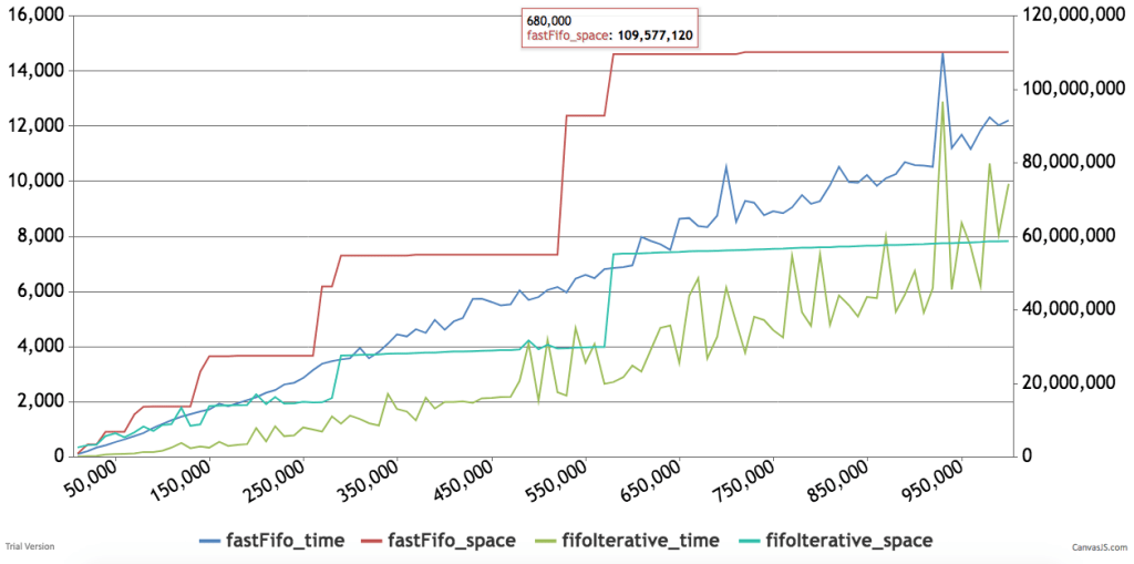
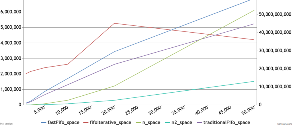
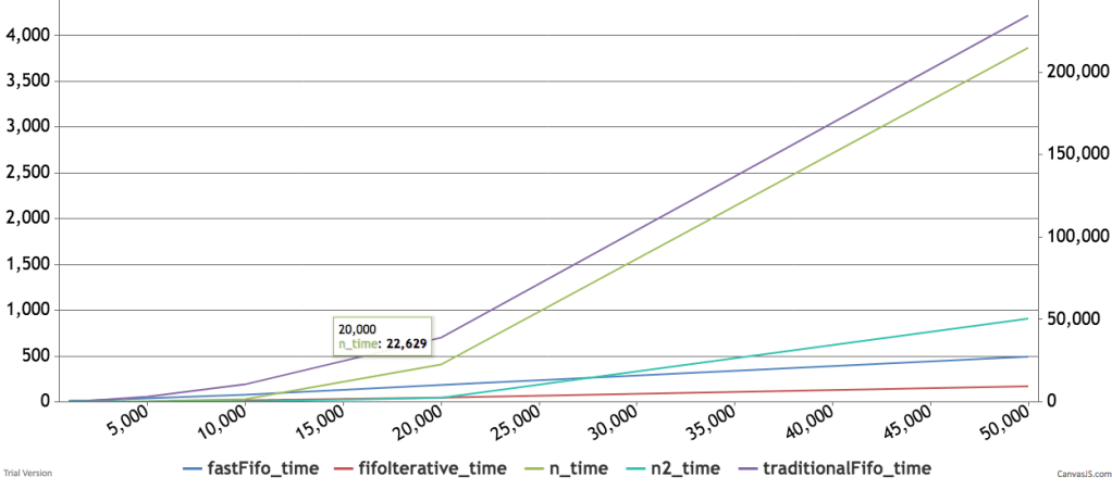
Below are some timings and graphs of memory usage. The code can be found here.

Evolutes
This next article was inspired by two sources:
An Advent of Code puzzle from 2017
An evolute is a matrix whose cells are numbered to spiral out from the center.
17  16  15  14  13
18   5   4   3  12
19   6   1   2  11
20   7   8   9  10
21  22  23---> ...
The first question asks us to find the Manhattan distance between some positive integer cell and the 1st cell.
I see two ways to do this:
- Build the evolute, find the location of the integer and then calculate the distance
- Calculate the coordinate with respect to the center directly and take the sum of the absolute value of the coordinates.
I will start with the second method because it is simpler. If we look at the structure of the evolute we will see that each new layer of the matrix will have an odd square in it’s bottom right corner. 1 9 25 49 ….
That means we can locate the layer by finding the nearest odd square root. Here is the code for that:
f:{j:floor sqrt x; j - not j mod 2}
q)f 10
3
q)f 25
5
q)f 24
3
Next we can find the grid coordinate or how far we are from the center for that corner. I plugged in max x so we can use the function on lists of numbers. The ‘?’ verb is being used to find index which corresponds to the steps away from the center.
g:{(1+2*til max x)?f x}
q)g 10
1
q)g 25
2
q)g 24
1
Now all we need to do is figure out where we are on the layer.
We can be in one of 5 places:
- Exactly at the end of a layer
- Between the bottom right corner and the top right corner
- Between the top right corner and the top left corner
- Between the top left corner and the bottom left corner
- Between the bottom left corner and the end of the layer
We can divide by the size of the layer to calculate this. We can also find the remainder to know how far between we are. This gives us the following code:
place:{(x-j*j) div 1+j:f x}
offset:{(x-j*j) mod 1+j:f x}
q)place 1+til 25
0 0 1 1 2 2 3 3 0 0 0 0 1 1 1 1 2 2 2 2 3 3 3 3 0
q)offset 1+til 25
0 1 0 1 0 1 0 1 0 1 2 3 0 1 2 3 0 1 2 3 0 1 2 3 0
This allows us to write the full function to calculate the coordinate. All we need to do is to check which of those conditions are met fill in the coordinates from g, plus the appropriate offset and correct sign.
coordinate:{[x]
    x:(),x;
    f:{j:floor sqrt x; j - not j mod 2};
    g:{(1+2til max x)?y};     place:{(x-yy) div 1+y};
    offset:{(x-yy) mod 1+y};      j:f x;     brc:x=jj;
     grid:g[x;j];
     p:place[x;j];
     o:offset[x;j];
    ?[brc;flip (grid;neg[grid]);
     ?[0=p;flip (grid+1;neg[grid]+o);
      ?[1=p;flip (grid+1-o;grid+1);
       ?[2=p;flip (neg[grid+1];1+grid-o);
        flip (neg[grid+1]+o;neg[1+grid])]]]]
    }
q)coordinate 1+til 9
0  0
1  1
1  1
0  1
-1 1
-1 0
-1 -1
0  -1
1  -1
At this point we can find the coordinate of any cell number. Since we can do this for all the points, we should be able to create the evolute for any dimension by generating all the coordinates and then shifting them to the appropriate column/row number and inserting them into that matrix. We can do this cleverly by sorting the row and column separately, since we want a particular orientation and sorting each of them corresponds to either a horizontal transposition or a vertical transposition.
evol:{t:`row`col!(x div 2)+flip cordinate j:1+til x*x; (x;x)#exec val from `col xdesc `row xasc flip update val:j from t}
q)evol 7
37 36 35 34 33 32 31
38 17 16 15 14 13 30
39 18 5  4  3  12 29
40 19 6  1  2  11 28
41 20 7  8  9  10 27
42 21 22 23 24 25 26
43 44 45 46 47 48 49
Now that we can create a evolute and we see that given an evolute we can find the coordinates, we also see that permuting the row and column indexes gives us different orientations. This leads us to see how Joey Tuttle/Eugene McDonnell created an evolute from scratch. Let’s raze an evolute:
q)raze evol 5
17 16 15 14 13 18 5 4 3 12 19 6 1 2 11 20 7 8 9 10 21 22 23 24 25
Now let us permute it by the magnitude and then look at the differences:
q)iasc raze evol 5
12 13 8 7 6 11 16 17 18 19 14 9 4 3 2 1 0 5 10 15 20 21 22 23 24
q)deltas iasc raze evol 5
12 1 -5 -1 -1 5 5 1 1 1 -5 -5 -5 -1 -1 -1 -1 5 5 5 5 1 1 1 1
q)deltas iasc raze evol 3
4 1 -3 -1 -1 3 3 1 1
We now see a pretty clear pattern. We are repeating a pattern of 1,neg x,-1,x.
Each time we are taking 2 elements from the pattern. We take an increasing number of them and continue until we take x elements in shot. Here is Eugene’s explanation translated into q
f:{-1+2*x}
g:{(-1;x;1;neg x)}
k:{(f x)#g x}
h:{1+til x}
j:{-1 _ raze 2#'h x}
l:{-1 rotate raze (j x)#'k x}
m:{iasc sums l x}
n:{(x;x)#m x}
q)f 5
9
q)g 5
- -1 5 1 -5
q)k 5
-1 5 1 -5 -1 5 1 -5 -1
q)h 5
1 2 3 4 5
q)j 5
1 1 2 2 3 3 4 4 5
q)l 5
-1 -1 5 1 1 -5 -5 -1 -1 -1 5 5 5 1 1 1 1 -5 -5 -5 -5 -1 -1 -1 -1
q)m 5
24 23 22 21 20 9 8 7 6 19 10 1 0 5 18 11 2 3 4 17 12 13 14 15 16
q)n 5
24 23 22 21 20
9  8  7  6  19
10 1  0  5  18
11 2  3  4  17
12 13 14 15 16
Combining this into function we get:
evolute:{(x;x)#iasc sums -1 rotate raze (-1 _ raze 2#'1+til x)#'(-1+2*x)#(1;neg x;-1;x)}
We can shorten it just a bit and make it a bit faster by seeing that grabbing parts j,k,l can make use of how kdb overloads ‘where’. In KDB ‘where’ gives you the indexes of the 1s in a boolean mask. For example:
q)where 101b
0 2
However, a little thought reveals that we are returning the index of the element the number at that index. So we return one 0, zero 1,one 2. Generalizing this, we can think that where of 1 2 3 should return one 0,two 1s and three 2s and indeed KDB does this.
q) where 1 2 3
0 1 1 2 2 2
Knowing this, we can rewrite j k and l, which make heavy use of each and remove all the razing.
I am going to show how I built this up.
q){((x-1)#2),1} 5
2 2 2 2 1
q){1+where ((x-1)#2),1} 5
1 1 2 2 3 3 4 4 5
q){(where 1+(where ((x-1)#2),1))} 5
0 1 2 2 3 3 4 4 4 5 5 5 6 6 6 6 7 7 7 7 8 8 8 8 8
q){(where 1+(where ((x-1)#2),1)) mod 4} 5 /so that we cycle
0 1 2 2 3 3 0 0 0 1 1 1 2 2 2 2 3 3 3 3 0 0 0 0 0
q){(1;neg x;-1;x)(where 1+(where ((x-1)#2),1)) mod 4} 5
1 -5 -1 -1 5 5 1 1 1 -5 -5 -5 -1 -1 -1 -1 5 5 5 5 1 1 1 1 1
q){-1 rotate (1;neg x;-1;x)(where 1+(where ((x-1)#2),1)) mod 4} 5
1 1 -5 -1 -1 5 5 1 1 1 -5 -5 -5 -1 -1 -1 -1 5 5 5 5 1 1 1 1
The last step recreates l. So the whole function using where looks like this:
evolute:{(x;x)#iasc sums -1 rotate (1;neg x;-1;x)(where 1+(where ((x-1)#2),1)) mod 4}
Part 2 of the advent of code is even more interesting. It describes us filling the spiral by summing the neighbors, the center square starts at 1. Here is the description from advent.
Then, in the same allocation order as shown above, they store the sum of the values in all adjacent squares, including diagonals.
So, the first few squares' values are chosen as follows:
Square1starts with the value1.
Square2has only one adjacent filled square (with value1), so it also stores1.
Square3has both of the above squares as neighbors and stores the sum of their values,2.
Square4has all three of the aforementioned squares as neighbors and stores the sum of their values,4.
Square5only has the first and fourth squares as neighbors, so it gets the value5.
Once a square is written, its value does not change. Therefore, the first few squares would receive the following values:
147  142  133  122   59
304    5    4    2   57
330   10    1    1   54
351   11   23   25   26
362  747  806--->   ...
What is the first value written that is larger than your puzzle input?
Now given our earlier coordinate function, we just need to add elements in into empty matrix of 0s and sum the neighbors at each step to determine what to add. First, let’s write the simple pieces of finding the neighbors and summing them. Then we will conquer the composition.
/To find the neighbors according to our rule,
/ we basically find the coordinates for (1..9)
/ then we can add to x pair so it's centered around that one
neighbors:{x+/:coordinate 1+til 9}
q)neighbors (1;0)
0  1
1  1
1  2
0  2
-1 2
-1 1
-1 0
0  0
1  0
/We need to shift our coordinate system depending on the size of the matrix
shift:{i:div[count x;2]; (i+y)}
q)shift[3 3#0;coordinate 5]
0 2
/calculate the sum of the neighbors
sumN:{sum over .[x] each neighbors y}
q)(1+evolute 5)
17 16 15 14 13
18 5  4  3  12
19 6  1  2  11
20 7  8  9  10
21 22 23 24 25
q)(1+evolute 5)[2;3]
2
/Manually sum the neghbors of 2
q)sum 4 3 12 1 2 11 8 9 10
60
q)sumN[1+evolute 5;(2;3)]
60
Okay, we are going to start with a matrix that has single 1 in the center.
center1:{.[(x;x)#0;(a;a:x div 2);:;1]} /we are ammending a 1 at the x div 2
q)center1  5
0 0 0 0 0
0 0 0 0 0
0 0 1 0 0
0 0 0 0 0
0 0 0 0 0
Now that we see how easy it is to amend an element at a particular index, we can combine this with the notion of a fold(over). The idea is that we will keep updating this matrix with new elements based on the neighbor sum:
cumEvolute:{{.[x;y;:;sumN[x;y]]}/[j;shift[j:center1[x]] coordinate 1+til (x*x)]}
q)cumEvolute 5
362 351 330 304 147
747 11  10  5   142
806 23  1   4   133
880 25  1   2   122
931 26  54  57  59
/If we want to rotate it we can simply reverse flip
q)reverse flip cumEvolute 5
147 142 133 122 59
304 5   4   2   57
330 10  1   1   54
351 11  23  25  26
362 747 806 880 931
Using cumEvolute we can find when we generate the first integer bigger than the input, by creating a stopping condition and counting the number of iterations.
stopCum:{{$[z<max over x;x;.[x;y;:;sumN[x;y]]]}/[j;shift[j:center1[x]] coordinate 1+til (x*x);y]}
q)stopCum[5;20]
0 0  0  0 0
0 11 10 5 0
0 23 1  4 0
0 0  1  2 0
0 0  0  0 0
q)max over stopCum[5;20]
23
q)max over stopCum[10;100]
122
As of Join Performance a surprising result
The Kx wiki describes in detail how to structure as of join queries for best performance.
https://code.kx.com/wiki/Reference/aj
3. There is no need to select on quote, i.e. irrespective of the number of quote records, use:
aj[`sym`time;select .. from trade where ..;quote]instead of
aj[`sym`time;select .. from trade where ..;
             select .. from quote where ..]
The reason for this is that since the quote table is partitioned on date and grouped on sym the as of join function simply scans the sectors of the disk in linear order and grabs the first matches using binary search.
Linear access to disk is very different from random access. So when you perform a search linearly on partitioned historical database it runs pretty fast.
However, someone asked me if you were going to query over and over, the same data whether then it made sense to do some pre-filtering on the quote table before doing multiple ajs.
At the time, I said it shouldn’t be faster. I thought that the overhead of reading from disk afresh each time was going to be much smaller than the overhead of allocating a very large amount of room in memory.
So I tested it:
taj1:{[t;d] now:.z.T;
do[10;aj[`sym`time;select from t where date=d;select from quote where date=d]]; after:.z.T;
after-now}taj2:{[t;d]
now:.z.T;
quotecache:select from quote where date=d, sym in exec sym from t; do[10;aj[`sym`time;select from t where date=d;quotecache]];
after:.z.T;
after-now}
The timings, were not even close the taj2, which precaches data when run 10 times, for a trade table with only 1000 records on only 100 symbols took more than 5 minutes to run. While taj1 was taking only 5 seconds, that is approximately 2 aj per second.
When I scaled the number of symbols to 1000, the cached version didn’t comeback and I had to cancel the query after 25 minutes. The non cached version took 10 seconds or 1 aj per second.
The intuition is correct, if you can prefilter, then not having to read in all the data twice should be faster. So I checked the meta of the cached table, it was loosing the p attribute while filtering.
I then created version taj3:
taj3:{[t;d]
now:.z.T;
quotecache:update `p#sym from select from quote where date=d, sym in exec sym from t;
do[10;aj[`sym`time;select from t where date=d;quotecache]];
after:.z.T;
after-now}
If you reapply the p attribute the first query for 1000 symbols costs you 3.6 seconds, but increasing the number of times you run the aj is almost free. So running 10 times only costs 4 seconds. Running 20 times the taj3 also took 4 seconds. So if you know you have a limited universe than reducing and pre-filtering is worth it if you will be running the queries again and again, JUST REMEMBER TO REAPPLY THE P ATTRIBUTE. Since the quote table is only filtered, the p attribute will be a really cheap operation, since order is preserved.
Q Idioms assemembered
This is more of an expanding list of Q idioms I have had to either assemble or remember or some combination.
- Cross product of two lists is faster in table form
q)show x:til 3
0 1 2
q)show y:2#7
7 7
q)x cross y
0 7
0 7
1 7
1 7
2 7
2 7
q) ([] x) cross ([] y)
x y
—
0 7
0 7
1 7
1 7
2 7
2 7
\t til[1000] cross 1000#5
85
\t flip value flip ([] til 1000) cross ([] x1:1000#5)
33
/and if you are happy working with it in table form
\t ([] til 1000) cross ([] x1:1000#5)
5
- Take last N observations for a column in a tableBoth of these can be used to create a list of indexes and the columns can be simply projected on to the list of indexes
/a) Intuitive way take last n from c
q) N:10; C:til 100000;
q) {[n;c]c{y-x}[til n] each til count c}[N;C] /timing 31 milli
0
1 0
2 1 0
3 2 1 0
4 3 2 1 0
….
/b) Faster way using xprev and flip
q) \t {[n;c] flip (1+til n) xprev \\: c}[10;c] /timing 9 millesec
- Create a Polynomial Function from the coefficients
poly:{[x] (‘)[wsum[x;];xexp/:[;til count x]]};
f:poly 0 1 2 3;
f til 5
0 6 34 102 228
- Count Non Null entries
All in K:
fastest:{(#x)-+/^x}
slower:{+/~^x}
slowest:{#*=^x}
Q translation:
fastest:{count[x]-sum null x}
slower:{sum not null x}
slowest:{count first group null x}
- Camel case char separated symbols:
camelCase:{[r;c]`$ssr[;r;””] each @'[h;i;:;]upper h @’ i:1+ss'[;r] h:string x}
most common case
q)c:` sv/: `a`b cross `e`fff`ggk cross `r`f
`a.e.r`a.e.f`a.fff.r`a.fff.f`a.ggk.r`a.ggk.f`b.e.r`b.e.f`b.fff.r`b.fff.f`b.ggk.r`b.ggk.f
camelCase[“.”;c]
`aER`aEF`aFffR`aFffF`aGgkR`aGgkF`bER`bEF`bFffR`bFffF`bGgkR`bGgkF
6. Progress style bars:
p:0;do[10; p+:1; system “sleep .1”;1 “\r “,p#”#”];-1 “”;
{[p]1 “\r “,(a#”#”),((75-a:7h$75*p%100)#” “),string[p],”%”;if[p=100;-1 “”;]}
7. AutoCorr:
autocorr:{x%first x:x{(y#x)$neg[y]#x}/:c-til c:count x-:avg x}
8. Index of distinct elements:
idistinct:{first each group x}
idistinct{x?distinct x}
9. index and transpose a matrix
{sv[x;::] y}
Tree Tables/Parent Vector representation of Dictionaries
Introduction:
http://archive.vector.org.uk/art10500340
Vector, the Journal of the British APL Association
TreeTables and the parent vector are magical things and they are a great way to flatten deeply nested structures. In particular, I will use this representation of a dictionary in the next post to allow you to import q libraries under a different namespace, kind of like what python allows with “import x as y”.
In this post I will focus on how we can easily rewrite a dictionary into a flat table with 4 columns. Let me motivate this a bit first. Take a deeply nested dictionary:
a| `b`c!(2;`d`e!(6;`f`g!7 8))
b| `c`d!4 5
c| `d`e!(6;`f`g!7 8)
In json that might look like this:
{
  "a":{
    "b":2,
    "c":{
      "d":6,
      "e":{
        "f":7,
        "g":8
      }
    }
  },
  "b":{
    "c":4,
    "d":5
  },
  "c":{
    "d":6,
    "e":{
      "f":7,
      "g":8
    }
  }
}
As we can see each key is a letter and each value is either another dictionary or a number. In q we can apply functions into these arbitrarily nested dictionaries provided all the values conform. So for example we can add 10+d
a| `b`c!(12;`d`e!(16;`f`g!17 18))
b| `c`d!14 15
c| `d`e!(16;`f`g!17 18)
However, once your dictionaries stop conforming things can get a bit hairy. As a simple example let’s add a simple dictionary f!f to the key f in d
a| `b`c!(2;`d`e!(6;`f`g!7 8))
b| `c`d!4 5
c| `d`e!(6;`f`g!7 8)
f| (,`f)!,`f
Suddenly 10+d throws a type error. Because we can’t add 10 to the non numeric dictionary. We can always right logic to avoid those cases, but it would be simpler to simply pull out all the conforming values add 10 to them and then replace them in the original structure. A tabular tree representation aids in this. As an example the same dictionary in tabular form: (I have omitted some results in the middle for ease of reading.) Which I will call treeTable:
l p c d
———
0 0 :: 1
1 0 `a 1
1 0 `b 1
1 0 `c 1
1 0 `f 1
2 1 `b 1
2 1 `c 1
…
4 15 8 0
5 21 7 0
5 22 8 0
The column c (child) contains every key and value, column d tells you if the row is leaf node or has a dictionary below it. Pulling out all the numeric children is as simple as:
numeric:6 7 8 9h
select c from treeTable where not d, (abs type each c) in numeric
c
-
2
4
5
6
6
7
8
7
8
This table can then be modified and assuming we can convert it back into its dictionary form we could then work with nested data easily.
How the Magic is done:
At this point you either believe this structure is useful or you believe it isn’t but you are still interested in understanding how this transformation happens.
Let’s look at the original treeTable and unpack the meaning of the columns.
The first column l represents the level of the dictionary that the key or value is located in.
The second column p is the index of the parent row in this table. The root of the table is self parenting meaning that the 0th row is at the 0th level and it’s parent is 0 (keep this in mind it will be useful in a second). All elements will have a parent.
The third column c is the child and it is the value at this level of nesting. It will either be a key if there are more levels below or it will just be the value at that level.
The fourth and final column d indicates whether or not this row is a dictionary. That is, whether the child should be treated as a key or a value.
To convert a dictionary into a treeTable we use breadth first search, that is the purpose of the l column. We first define a primitive treeTable with only one row the root.
l p  c  d
---------
0 0  :: 1
All treeTables will have this row. If the thing we are trying to convert into a treeTable is not a dictionary but is instead SOMEKIND_OF_THING_THAT_IS_NOT_A_DICTIONARY. Then there will be only one more row in this table.
l p  c  d
---------
0 0  :: 1
1 0 SOMEKIND_OF_THING_THAT_IS_NOT_A_DICTIONARY 0
We will then know we are done because there are no more dictionaries to unpack at the last level.
If instead we get a dictionary. We will first record all the keys at that first level and return the table.
Our ability to find a value at a particular level is enabled through the use of the parent column in the treeTable. Suppose we have a simple dictionary:
{
 "d":6,
 "e":{
   "f":7,
   "g":8
  }
}
We can record this as the following two columns:
p c index
----------
0 :: 0
0 `d 1
0 `e 2
2 `f 3
2 `g 4
1  6 5
3  7 6
4  8 7
The first row is the root it is self parenting. The next two rows are both top level keys. So their parent is the root. f and g both are under e so their parent is 2, but 6 is under d so it’s parent is 1. To make this easier to see, I have added the virtual index column which is always available. Then the final two rows are under f and g respectively.
If we want the parent of particular row, and we have the parent column, which I will call p:0 0 0 2 2 1 3 4
We can index into that row to get the parent. p 6 -> 3 which is f
We can repeat this until we get to the root. p 3 -> 2; p 2-> 0 ; p 0 -> 0. To find the root in one step we can use KDB’s built-in converge function which will apply until two consecutive results are the same. This is why it was so convenient for the root to be self-parenting. So see the path to the root use scan instead of over.
p over 6 -> 0
p scan 6 -> 3 2 0. Now that we have a path, we just need to get the keys that correspond to that path, this is done by indexing the path against the child column.
c 3 2 0 -> f e ::
We now can get the unique path to any element.
The next step is using the path to index into any level of the dictionary. This is accomplished with a special object called getItems.
getItems is defined by combining the indexing at depth verb with a function that reverses the path list and checks if the path list happens to be only the root. In which case, we simply return the original item.
Using just those two ideas, we are able to construct the treeTable. The algorithm is to index one level at a time each time recording the if the level contains dictionaries or not. If it contains no dictionaries we are done and we will return the same table twice in row, which means that our function will converge. Using breadth first search we avoid any stackoverflow issues that could happen with a recursive solution, instead the function becomes tail recursive, meaning all the necessary ingredients to call the function again are returned as the output. That is why on the first call the function returns the first row of a treeTable. That way each call after simply indexes deeper into the original dictionary to return more levels of the treeTable.
The Code and An Example:
toTreeTable:{[d]
 getItems:('[;] over (.[d;];{$[x~(enlist[::]);x;1_reverse x]}));
 tTT:{[getItems;t]
 $[98h~type t;;t:([]l:(1#0);p:0;c:(::);d:1b)];
 lev:last t[`l];
 k:exec i from t where l=lev,d;
 $[count k;;:t];
 paths:t[`c] (t[`p]\')k;
 items:getItems each paths;
 id:where bd:99h=type each items;
 p:raze (count each key each items[id])#'k[id];
 c:raze key each items[id];
 df:count[p]#1b;
 lvl:count[p]#lev+1;
 id:where not bd;
 p:p,k[id];
 c:c,items[id];
 df:df,count[id]#0b;
 lvl:lvl,count[id]#lev+1;
 t upsert flip `l`p`c`d!(lvl;p;c;df)}[getItems];
 tTT over ()}


/an example of a nested structure


b:`c`d!4 5
e:`f`g!7 8
c:`d`e!(6;e)
a:`b`c!(2; c)
d:`a`b`c!(a;b;c)
q)toTreeTable d
l p c d
---------
0 0 :: 1
1 0 `a 1
1 0 `b 1
1 0 `c 1
2 1 `b 1
2 1 `c 1
2 2 `c 1
2 2 `d 1
2 3 `d 1
2 3 `e 1
3 5 `d 1
3 5 `e 1
3 9 `f 1
3 9 `g 1
3 4 2 0
3 6 4 0
3 7 5 0
3 8 6 0
4 11 `f 1
4 11 `g 1
4 10 6 0
4 12 7 0
4 13 8 0
5 18 7 0
5 19 8 0
And Back Again!
Now that we covered how to get a treeTable we can also understand how to go back to a dictionary.
We apply the opposite approach. The core function returns a dictionary. Each time we return a dictionary that is slightly deeper than the previous time. We put placeholder empty dictionaries until we build the final result. Since we know whether each row is a key or a value, we know whether the current item requires a placeholder.
toDictFromTreeTable:{[tt]
 tD:{[tt;dSoFar;lev]
 dS:exec {x!count[x]#enlist[()!()]}[c] by p from tt where l=lev, d;
 dS:dS,.[!; value exec p,c from tt where l=lev, not d];
 pR:tt[`c](-1_|:) each (tt[`p]\')[key dS];
 pC:tt[`c]key dS;
 paths:raze each {(1_x;enlist[y])}'[pR;pC];
 $[lev>1;.[;;:;]/[dSoFar;paths;value dS];first value dS]}[tt];
 tD/[()!();1+til last tt[`l]]}
Wow This is Even More General Than We Thought:
When I first built this, I tried to make sure that I covered simple dictionaries and values. So I was curious what would happen to keyed tables. Keyed tables are special in that they are essentially dictionaries whose key and values are both dictionaries. Since a dictionary is a pair of lists and a list of dictionaries is a table. A keyed table is simply a dictionary whose key is a table and and whose value is a table. A trivial example to illustrate this point:
q)k:([]k:til 5)
k
-
0
1
2
3
4
q)v:([]v:10*til 5)
v
--
0
10
20
30
40
q)kv:k!v
k| v
-| --
0| 0
1| 10
2| 20
3| 30
4| 40
/Indexing against the key table returns the value table
q)kv[k]
v
--
0
10
20
30
40
/but we can also apply select only certain rows using the k column
/in this case I reverse the key table and take the first 2 rows.
q)kv[2#reverse k]
v
--
40
30
Now what happens if we turn a key table into a treeTable:
l p c d
---------------
0 0 :: 1
1 0 (,`k)!,0 1
1 0 (,`k)!,1 1
1 0 (,`k)!,2 1
1 0 (,`k)!,3 1
1 0 (,`k)!,4 1
2 1 `v 1
2 2 `v 1
2 3 `v 1
2 4 `v 1
2 5 `v 1
3 6 0 0
3 7 10 0
3 8 20 0
3 9 30 0
3 10 40 0
It converts the key part of the table into key dictionaries that are the parents of the value dictionaries in the table. And we can turn it back:
q)toDictFromTreeTable toTreeTable kv
k| v
-| --
0| 0
1| 10
2| 20
3| 30
4| 40
q)kv ~toDictFromTreeTable toTreeTable kv
1b
In other words, keyedTables are treated like dictionaries, this means that if you only want to look at values, you will only see values, simply by select from the treeTable where not d. The internal dictionaries inside a keyed table are broken apart into their component dictionaries and the values are stored independently.
Tables Get Treated as singletons.
Since tables are actually lists of dictionaries, and lists are treated as values. A table is also treated as a value and placed directly into the child column.
q)t:([] til 10)
x
-
0
1
2
3
4
5
6
7
8
9
q)toTreeTable t
l p c d
---------------------------------
0 0 :: 1
1 0 +(,`x)!,0 1 2 3 4 5 6 7 8 9 0
The function from TreeTable correctly undoes the toTreeTable function
but the treeTable form is actually more nested than the original table.
q)toDictFromTreeTable toTreeTable t
x
-
0
1
2
3
4
5
6
7
8
9
We can fix this by expanding our parent vector to notate whether a current element is a dictionary, list or an atom. That way we would create a node that is the head of every list and then iterate through the indexes in the list. This is left as an exercise, or until I need this functionality.
