Every home cook knows that to get that extra dose of flavor, one needs to toast their spices like all the professionals. I’m here to tell you this not only unnecessary it’s counter productive.
The stated reason for this practice is that it release the aromatics makes the spices that much more potent. If you stop to consider this, it’s obvious why this makes no sense. Once the aromatics have been released they will float away and indeed the kitchen smelling amazing is proof that indeed that the aromatic oils are busy floating away, never to be seen or heard from again. If you want your kitchen to smell good, toast your spices. If on the other hand you want your guests to enjoy flavorful food, don’t toast the spices, instead heat your spices together with the food, especially food that has either oil or water which will bond to the flavorful aromatics and be released when the food is being chewed.
One goal of cooking with spices is to move the flavorful compounds from one ingredient to another (ie from the coriander seed to your chicken ). If you simply toast the spices the flavor will move from your pan into the oil that you toasted the spices in and into the kitchen air which while delicious for the cook does nothing for the guest.
Of course you can create delicious infusions by heating spices in oil and then using the oil to coat the food, but even that is better accomplished with a bit more oil and gentle heat. Sure there are certain flavor reactions you can get from toasting, essentially various Maillard reactions, but there are better ways to achieve that on a larger surface area of your food then on the poor spices which make up about 1% of a dish. Someone may point to an obvious counter example like toasted sesame seeds which taste nothing like sesame seeds. This is true, certain seeds completely change the flavor profile after being heated, but even that flavor is better imparted with a bit of toasted sesame oil. So why do chefs keep recommending this technique. The extra step is rather annoying and requires attention/technique – spices burn very quickly – and it makes the surrounding kitchen smell amazing so it must be what it’s imparting that delicious aroma into the food.
Street vendors toast spices as advertising, it’s easy to get customers to be excited about a dish if the cart smells really good, a bit of wasted aromatics into the street air are worth every penny if it draws customers in.
Author: pindash91
An argument for the direct approach
Recently, I solved a very minor problem and introduced a regression. Sure the tests caught this regression but the bug didn’t need to be coded at all. The direct approach skips the bugs. That’s the argument.
Since you’re still reading, I’ll walk you through my thought process how I came to make the mistakes and how a moment away from the keyboard gave me enough perspective to see the solution clearly.
I work with US equities and I have jobs that run on a schedule they essentially pull data in near realtime do some analytics and display the data on a dashboard. The minor problem was that data technically doesn’t get updated after the market closes. So that creates a good time for maintenance tasks to be run on the database. Ideally, this means no one is querying the database unless they need something, this makes it much easier since you don’t need to ask or let anyone know that the database is going down, you simply wait for the last query to finish and then perform the maintenance tasks. While prototyping it was much easier to pull the data round the clock. So the task was simple change all the jobs to pause overnight.
The jobs were scheduled inside a very primitive cron library. So naturally the idea was to simply add two cron jobs. One cron would remove the jobs at night and another cron add the jobs back the next day.
The bug was introduced, because having a job that schedules itself to run can create a cycle. Since the job that adds jobs must be run in the morning, it naturally has a higher time priority and so it can call itself over and over.
However, the better solution is to simply add one cron, which runs daily at the end of the day and simply pushes all the timers forward to the next day. This takes care of having to register all the jobs in some function that is responsible for scheduling intraday jobs. There is one less cron to worry about and the effect is just another cron which happens to essentially sleep all activity at night.
Why did I not think of the first approach, because I was using the API provided by the library, the library didn’t have a way to delay all current timers, but the implementation was simple every job had a scheduled run time and if the clock crossed the set time the job was eligible to be run at which point it would be pulled off the queue and ran and then a policy would be invoked to schedule it again. This policy approach allows the library to handle periodic retries/ exponential backoff/ uniform repeat/ one and done/ crontab syntax. The implementation of the next run time allows all jobs to be delayed. Max all scheduled times that are scheduled after the sleep time with the new scheduled time in the future. This will push jobs between now and the wake time to after the wake time and won’t affect jobs scheduled after the wake time, it will also ensure that jobs intended to run before night will still run.
Can you think of cons to this approach sure:
- The timer implementation has now been leaked
- Jobs that are supposed to run at night won’t run until the morning
- The next run time is now some combination of the policy and a random job
These are all valid reasons to adopt a more elaborate approach perhaps even write your own custom policy and add it to the cron library. Resist that urge, (I say to myself as much as to you dear reader) you ain’t gonna need it (I’ll post an update and eat my words if I ever need to implement a custom policy). The process feeds data to a dashboard that is monitored around trading hours, going to sleep at night is precisely what is called for. Anything scheduled during nighttime hours can be safely pushed to the morning.
If you think the example is too contrived, it is indeed a didactical example, but sadly all too real.
Maybe your unconvinced, if so why?
Vector thinking for Max Profit
Occasionally I am lucky enough to run into a problem that doesn’t already have many vector solutions, so I can demonstrate how vector thinking can allow you to find an elegant solution. To build up to my insight let’s solve 2 easy variations and then we can get to the two more interesting puzzles.
The problem in question is called Best Time to Buy and Sell or more popularly simply Max Profit.
The theme is always the same you are given an ordered list of positive numbers that represent the evolution of the price of the security. You must find the maximum profit you could have made given this price series. You can only hold 1 unit at a time and you can not short, which means you must buy before you can sell (you can only profit from the price evolving upward).
The simplest and most well know variation is the 1 transaction problem (leetcode problem 121): you can only buy and sell at most 1 time what is the max profit that can be earned from the following series:
example series:
3 2 5 1 3 2 4 9 5 12 3 5
The key insight into this problem is that we are looking for the largest difference between the current element and the smallest element we have seen.
To motivate this insight, let’s look at ever larger versions of this problem starting with just one price to detect the pattern.
3 -> 0
Given just one price we can only buy and sell on the same day, so effectively max profit is 0
3 2 -> 0
Given these two points we can still only earn 0, since we must sell after we buy.
3 2 5 -> 3
Now that we have a higher number after a lower number we can plainly see that of the two options buy at 3 or buy at 2, buy at 2 and sell at 5 is better.
3 2 5 1 -> 3
The answer is still 3, since we can’t sell higher than 5, and even if we bought at 1 at the end there are no days left to sell
3 2 5 1 3 -> 3
We still do best by buying at 2 and selling at 5, buying at 1 and selling at 3 only earns 2.
3 2 5 1 3 2 -> 3
Plainly the 2 at the end doesn’t improve
3 2 5 1 3 2 4 -> 3
We can now either buy at 2 and sell at 5 or buy at 1 and sell at 4, but our max profit is still 3.
3 2 5 1 3 2 4 9 -> 8
Finally, the max profit changes! We can now buy at 1 and sell at 9. As new elements are added the new reward will be a function of the lowest element seen thus far.
We then get our solution:
{max x-mins x} 3 2 5 1 3 2 4 9 5 12 3 5
11, where we buy at 1 and sell at 12.
Or in python we could say something like:
import itertools
from operator import sub
def max_profit(p):
    return max(map(sub,p,itertools.accumulate(p,min)))
To unpack this a bit, mins returns the min element up to that point:
mins[3 2 5 1 3 2 4 9 5 12 3 5]
3 2 2 1 1 1 1 1 1 1 1 1
we can then do element-wise subtraction to see what the profit is from selling at each point
0 0 3 0 2 1 3 8 4 11 2 4
taking the running max we get the max profit so far,
0 0 3 3 3 3 3 8 8 11 11 11
we can see that this series is exactly the results that we got when we were looking at the max profit for the prefixes of the series.
Easy enough, let’s look at version 2 of this problem (leetcode 122):
unlimited number of transactions: We are now allowed to buy and sell as often as we like provided we never own more than 1 share of the stock and we still must sell after we bought. To make things easier we can assume that we can buy and sell on the same day, in practice this doesn’t matter as any day we do this we can consider that we did nothing.
Keeping the same price series as before:
3 2 5 1 3 2 4 9 5 12 3 5
We now notice that we should take advantage of every single time the price goes up. Again let’s look at a smaller example to get some intuition.
3 2 5 -> 3
Nothing fancy here, we buy at 2 and sell at 5, purchasing at 3 doesn’t improve our profit since selling at 2 would incur a loss.
3 2 5 1 3 -> 5
buy at 2 sell at 5, buy at 1 sell at 3
3 2 5 1 3 2 4 -> 7
just add one more purchase at 2 and sell at 4,
3 2 5 1 3 2 4 9 -> 12
Here it becomes interesting, we can look at two interpretations
buy at 2 sell at 5 (3),buy at 1 sell at 3 (2), buy 2 sell at 9 (7) for a total of 12
or we can say:
buy at 2 sell at 5 (3),buy at 1 sell at 3 (2), buy at 2 sell at 4 (2),buy at 4 sell at 9 (5) for a total of 12.
The two approaches are identical since addition commutes, it doesn’t matter how you get from 2 – 9 you will always earn 7.
Which means that we can simply add up the positive steps in the price series. That will be the maximum profit for an unlimited number of transactions:
Our code is simply:
{(x>0) wsum x:1 _ deltas x} 3 2 5 1 3 2 4 9 5 12 3 5
21
Deltas gives us the adjacent differences. We drop the first delta since we cannot sell before we have bought. If the delta is positive >0 we want to include it in our sum. Using (w)eighted(sum) we weight the >0 with a 1 and less then 0 or =0 are given a weight of 0.
Now that we covered the case with 1 transaction and unlimited transactions, we should feel confident that we can tackle 2 transactions. Lucky for us, that’s exactly version III of the problem (leetcode 123):
Getting insight into how to solve this variation should start with thinking about how we could solve this naively. The correct heuristic to reach for is divide and conquer. Suppose that for every step along the price evolution we knew what the max profit was before and the max profit was after. Then we could sum those two max profits and take the largest combination.
assume max_profit function as before:
r=range(len(p))
max([max_profit(p[0:i])+max_profit(p[i:]) for i in r)])
For our example this gives us 15.
What we might notice is that we are recomputing the max profit over for larger and larger prefixes, and for smaller and smaller suffixes.
We know that the prefixes were already computed simply by taking the rolling max instead of the overall max in max_profit. The only thing we’re missing is how to calculate the max_profit of suffixes.
Now we notice a symmetry – while the prefixes are governed by the rolling minimum, the suffixes are bounded by the rolling maximum from the left, i.e. the largest element available at the end to sell into.
To get a sense of this, look at the solutions to the suffixes
3 5 -> 2 (buy at 3 sell at 5)
12 3 5 -> 2 (buy at 3 sell at 5)
5 12 3 5 -> 7 (buy at 5 sell at 12)
9 5 12 3 5 -> 7 (buy at 5 sell at 12)
4 9 5 12 3 5 -> 8 (buy at 4 sell at 12)
Which leads to this solution in q:
{max reverse[maxs maxs[x]-x:reverse x]+maxs x-mins x}
maxs x -mins x / is familiar from earlier
If we want to walk backwards through a list, we can reverse the list and apply the logic forwards then reverse the result, which is the same as applying the logic to the suffixes.
So all we need to do is to subtract each element from the running maximum then take the running max of this result to get the max profit for the suffix so far.
In Python this simply becomes:
from itertools import accumulate as acc
from operator import add,sub
def max_profit_2trans(p):
    before=list(acc(map(sub,p,acc( p,min)),max))
    p.reverse()
    after=list(acc(map(sub,acc(p,max),p),max))
    after.reverse()
return max(map(add,b,a))
Alright, finally we should be able to tackle the most general version of this problem (leetcode 188). You are given both a series of prices and allowed to make up to k transactions. Obviously, if k is 1, we solved that first. We just solved k is 2. You can verify for yourself, but if k is larger than half the length of the price series the max is the same as the second problem we solved. Since every pair of days can allow for at most one transaction, effectively k is unlimited at that point.
We need to solve the k>2 but less than k<n/2. The standard CS technique that comes to mind is some kind of dynamic programming approach. To quote MIT’s Erik Demaine CS6006 dynamic programing is recursion plus memoization.
Let’s setup the recursive solution and assume we are at a particular (i)ndex in our price series, with k transactions left.
Let’s start with the base cases:
If k equals 0 we return 0
If i is greater than the last index, i.e. there are no elements left in the list: we return 0.
Otherwise the solution to the problem is simply the maximum of 2 options:
do nothing at this step:
0+the function increment i
do something:
If we are (h)olding a share we can sell at this step which adds the current price +the result of this function with one less k and i incremented by 1.
Otherwise we buy at this step, which is minus the current price (we spend money to buy) plus the result of this function with i incremented and we are now holding a share.
Here is the code for this in q:
p:3 2 5 1 3 2 4 9 5 12 3 5
cache:(0b,'0,'til[count p])!count[p]#0
f:{[h;k;i]$[i=count p;0;(h;k;i) in key cache;cache[(h;k;i)];
:cache[(h;k;i)]:.z.s[h;k;i+1]|$[h;p[i]+.z.s[0b;k-1;i+1];.z.s[1b;k;i+1]-p i]]}

We can test this and see that it results in the right answer for k=0,1,2
f[0b;0;0] -> 0 no surprise with 0 transaction no profit is possible
f[0b;1;0] -> 11 the original problem
f[0b;2;0] -> 15 buy at 1, sell at 9, buy at 5 sell at 12
However, we know that a vector solution is possible for k=1,2,infinity, so we might hope there is a vector solution for when k is 3 and above.
We can analyze the intermediate results of the cache to get some sense of this.
code to look at the table
t:(flip `h`k`j!flip key cache)!([]v:value cache)
exec (`$string[j])!v by k from t where not h
output table:
 | 11 10 9 8 7 6  5  4  3  2  1  0
-| --------------------------------
0| 0  0  0 0 0 0  0  0  0  0  0  0
1| 0  2  2 7 7 8  10 10 11 11 11 11
2| 0  2  2 9 9 12 14 14 15 15 15 15
3| 0  2  2 9 9 14 16 16 17 17 18 18
4| 0  2  2 9 9 14 16 16 18 18 20 20
What we might notice is that the first row is the running maximum from selling at the prefixes. Then it’s the combination of the previous row and 1 additional transaction. In other words, each row allows you to spend money from the previous row and sell at the current price.
Putting this into action we get the following:
{[k;p]last {maxs x+maxs y-x}[p]/[k;p*0]}
We can look at intermediate rows by writing the scan version of the code and we know it will converge to the unlimited transaction case:
{[p]{maxs x+maxs y-x}[p]\[p*0]} p
0 0 0 0 0 0 0 0  0  0  0  0
0 0 3 3 3 3 3 8  8  11 11 11
0 0 3 3 5 5 6 11 11 15 15 15
0 0 3 3 5 5 7 12 12 18 18 18
0 0 3 3 5 5 7 12 12 19 19 20
0 0 3 3 5 5 7 12 12 19 19 21
What’s really nice about this code is that it actually describes the problem quite well to the computer and in effect finds exactly what we want.
p*0 / assume we have 0 transactions and therefore 0 dollars at each step.
y-x / subtract the current price(x) from the current profit(y) element wise
maxs y-x/ find the rolling max revenue
x+maxs y-x / add back the current selling price
maxs x + maxs y-x / find the rolling max profit
repeating this k times finds the max profit of the k’th transaction.
Here is the python code that implements this logic:
import itertools
from operator import add,sub
def max_profit(k: int, prices: List[int]) -> int:
        if k==0 or len(prices)<2:
            return 0
        z=[0]*len(prices)
        maxs=lambda x: itertools.accumulate(x,max)
        addeach=lambda x,y: map(add,x,y)
        subeach=lambda x,y: map(sub,x,y)
        for i in range(k):
            z=maxs(addeach(prices,maxs(subeach(z,prices))))
        return list(z)[-1]
I think this post covers this puzzle, let me know if there are interesting variations I haven’t explored.
Idempotent + Moving Window is simply a reduction
I want to calculate the moving window max or min in a data parallel way.
Lets start with the two argument function max
max(x,y) returns the greater of x and y
max(x,x) returns x (idempotent)
max(5,3) return 5
max(max(5,3),max(5,3)) reduces to max(5,5) which just returns 5
If we want max of an entire list we can simply think of it as a reduction in the lisp/APL sense
max(head (x), (max (head (tail (x), max( head(tail(tail(x))), …. )
or in a more readable way, replace max with |, and insert it between every element in the list
x[0] | x[1] | x[2] | x[3] this is a standard reduction/over.
Here is a concrete example:
x:5 4 3 2 7 2 9 1
Max over(x) –> 9
|/x –> 9
We can look at the intermediate results
Max scan(x) –> 5 5 5 5 7 7 9 9
|\x –> 5 5 5 5 7 7 9 9
Now let’s say that we want to look at the 3 slice moving window.
Let’s take advantage of the fact that max(x,x) yields x, idempotent
We can calculate the max between each pair in our list. Read max each-prior (‘:)
(|’:)x –> 5 5 4 3 7 7 9 9
applying this function n-1 times gives us a moving max
so (|’:) (|’:) x is 3 slice moving window, which we can rewrite as
2 |’:/ x
5 5 5 4 7 7 9 9
We can see that |\x is equivalent to (count[x]-1) |’:/ x which is data parallel by construction. In other words, we are doing an adjacent transform.
To make this a bit clearer, we can show intermediate results by using a scan(\) instead of an over(/)
(count[x]-1)|’:\x
5 4 3 2 7 2 9 1
5 5 4 3 7 7 9 9
5 5 5 4 7 7 9 9
5 5 5 5 7 7 9 9
5 5 5 5 7 7 9 9
5 5 5 5 7 7 9 9
5 5 5 5 7 7 9 9
5 5 5 5 7 7 9 9
One thing we can notice is that we could terminate early, since we know that if an adjacent element did not change there is no way for the max value to propagate further.
Which means we can rewrite (count[x]-1)|’:\x to simply (|’:\)x
and indeed this gives us:
(|’:\)x
5 4 3 2 7 2 9 1
5 5 4 3 7 7 9 9
5 5 5 4 7 7 9 9
5 5 5 5 7 7 9 9
Technically this is still slower than maxs(x) but if we had gpu support for each-prior(‘:) we could calculate maxs in n calls to max prior which has a parallelization factor of n/2. Depending on the range of x, the n calls might be bound significantly such that for small ranges, for example you are dealing with a short int (8 bytes), you can effectively compute the maxs in O(c*n/2) time with parallelism. Where c is a function of the effective range of your inputs — max[x]-min[x].
Now let’s get back to the problem of max in a sliding window, like this leetcode problem. This problem is classified as hard and the reason is that leetcode doesn’t want you to use parallelism to solve sliding window, it wants you to do it in O(n) time directly.
We know we can solve the problem in O(n) time when the window is equal to 1,2, and n.
identity({x}), max each prior ({|’:x}), and maxs ({|\x}) respectively.
The key to solving it for all window sizes is to recognize that each entry only depends on itself and its neighbors and that the result is the same if you duplicate neighbors – again idempotentcy comes to the rescue. max(1 2 3) is equal to max(1 1 2 2 3 3). Another good explanation can be found here. This is technically a dynamic programming approach with two pointers, but I have never seen it explained in what I think is the most straightforward way.
Let’s borrow the example from leetcode and work through what should happen.
Suppose list of numbers n=1 4 3 0 5 2 6 7 and window size k=3. Then reusing the prior code to show intermediate steps, we get:
1 4 3 0 5 2 6 7
1 4 4 3 5 5 6 7
1 4 4 4 5 5 6 7
If we look at a particular slot, 0 for example, it gets overtaken by 4, but the 5 slot only needs to compete with 3. In other words, each element is looking at at most n-1 elements to the right and n-1 elements to the left. So we can rearrange n to do this in a natural way. Let’s reshape n, so that there are k columns. q supports ragged arrays, so our last row is not the same length which is nice.
q)(0N;k)#n
1 4 3
0 5 2
6 7
We can then compute the maxs of each row
q)maxs each (0N;k)#n
1 4 4
0 5 5
6 7
And flatten it back:
q)l:raze maxs each (0N;k)#n
q)l
1 4 4 0 5 5 6 7
This gives us our left window. Now we will repeat the steps but instead of going from the left we will go from the right.
The simplest way go from the right is to reverse the list apply the function as normal from the left and reverse the list again. In J this operation is called under, as in going under anesthesia, perform the operation and then wake you from the anesthesia. This is equivalent to looking at the cummulative max from the right or walking backward through the array.
q)under:{[f;g](f g f ::)}
q)(reverse maxs reverse)~under[reverse;maxs] /this is the same
1b
q)(reverse maxs reverse ::) each (0N;k)#n
4 4 3
5 5 2
7 7
Now we just need to flatten the list and call it r.
q)r:raze (reverse maxs reverse ::) each (0N;k)#n
Because r is going from the right, we need to shift it by k-1 elements to the right so that we are not using data from the future when looking at what the current max should be. Printing l on top of r, we get:
q)(l;(k-1) xprev r)
1  4  4 0 5 5 6 7
0N 0N 4 4 3 5 5 2
As we can see, a simple max along the columns will give us the correct answer. (Note: the 0N in the beginning correspond to nulls)
q)max (l;(k-1) xprev r)
1 4 4 4 5 5 6 7
This idea can be generalized, so let’s write a generic function that can take an idempotent operation and create a moving window version.
fmx:{[f;g;h;m;x]l:raze (f')w:(0N;m)#x;r:raze (g')w;h[l;(m-1) xprev r]}
fmx takes a function f that will be applied to generate the left window, a function g that will be used to generate the right window and h a function that will combine left and right windows shifting r based on the window.
We can now generate (mmax, mmin, mfill):fmmax:fmx[maxs;(reverse maxs reverse ::);|]
fmmin:fmx[mins;(reverse mins reverse ::);{&[x;x^y]}] /fill the nulls with x
fmfill:fmx[fills;(reverse ({y^x}) reverse ::);{y^x}]
We can also generate a function that will allow us to inspect what elements we have access to in the right and left windows so that we can debug/make new functions, with some small modifications.
inspect:fmx[,\;(reverse (,\) reverse ::);{([]l:x;r:y)}]
Here we define f to concatenate the elements seen so far, g is the reverse concatenate, and h is return a table of the l and r.
When we run inspect on our original n, we see that every row has the information from the appropriate sliding window in it, though sometimes more than once.
q)inspect[k;n]
l      r
--------------
,1     `long$()
1 4    `long$()
1 4 3  1 4 3
,0     4 3
0 5    3
0 5 2  0 5 2
,6     5 2
6 7    2
We can see that the combination of left and right windows will always have at least the three elements required.
To summarize, we saw that idempotent functions, like max and min, allow for parallelization and allow us to use the dynamic programming two pointer technique to solve sliding window calculation in O(n).
Below is the python code for sliding maximum window, written in numpy/APL style, I’m not sure it makes the concept clearer, but more people read python than q. numpy doesn’t like ragged arrays, so there is a bit of extra code to handle the cases where count of n is not evenly divisible by k.
def maxSlidingWindow(k,nums)
  cmax=np.maximum.accumulate
  n=len(nums)
  z=np.zeros(k*np.ceil(n/k).astype(int))
  z[:n]=nums
  z=z.reshape(-1,k)
  l=np.resize(cmax(z,1).reshape(z.size),n)
  r=np.resize(np.flip(cmax(np.flip(z,1),1),1).reshape(z.size),n)
  return list(np.max(np.stack([l[k-1:],r[:r.size-(k-1)]]),0).astype(int))
all code can be found here:
https://github.com/pindash/q_misc/blob/master/sliding_window_max.q
Terse Code
According to this nature article additive solutions are preferred to subtractive solutions. This heuristic may encode a form of Chesterton’s fence, but it blinds people to finding solutions that are better by taking for granted what is. The article says people don’t dismiss the subtractive solutions, rather they never consider them in the first place. The idea behind terse code, may simply reverse this heuristic thus opening the mind to novel connections that would be hidden by a strictly additive approach. This might explain why constraints are so often a boon to creativity. They take the place of the mind’s general purpose heuristics in narrowing the search space, but leave open areas pertinent to the problem. So for example, trying to fit a piece of code into n chars, forces the user to rethink complicated methodologies and solve just the core problem. Other constraints that work similarly are constraints on performance, usually solutions that achieve 80% or more of the result can be achieved by simplifying the objective. Such bouts of creativity only come from constraining the resources that can be marshaled at a given task. A great example of this is the SVM technique used early to recognize hand written addresses by the US post office. The computing power and training sets available were a small fraction of what we have today. Neural networks are a counter example, they seem to work better as they get larger. Perhaps that explains our own bias, or we might discover that some constraint on the networks yields vast improvements, only time will tell. My sympathies lie with occam.
Stable Marriage in Q/KDB
A friend of mine is applying to Medical Residency programs, which motivated me to investigate the matching algorithm used to match residents with hospitals. NRMP the organization behind the matching process has a dedicated video explaining how the algorithm works. The simplest version of the problem can be thought to consist of n guys and n gals who are looking to pair off. Each gal has a ranked list of guys and each guy a ranked list of gals. We want to find a pairing such that no guy and gal can pair off and be better off. We call this stable, since any gal who wants to leave can’t find a guy who isn’t currently happier with someone else. It takes two to tango, or in this case disrupt a stable pairing.
Gale-Shapley published a result on this problem in 1962 showed a few amazing properties:
- A stable pairing always exists
- There is an algorithm to get to this pairing in O(n^2)
- It is truthful from the proposing side, i.e. if men are proposing then they can’t misrepresent their preferences and achieve a better match
- The proposing side gets the best stable solution and reviewing side gets the worst stable solution
- The reviewing side could misrepresent their preferences and achieve a better outcome
Knuth wrote about this problem pretty extensively in a French manuscript. The University of Glasgow has become a hub for this problem, Professor Emeritus Robert Irving wrote the book on the topic and his student David Manlove has written another. New variations and approaches keep coming out, so in a way this problem is still an active area of research. For this post I want to look at only the simplest version and describe a vectorized implementation.
First let’s walk through an example by hand (note: lowercase letters are men)
Men ranking women
d| `D`B`C
b| `B`C`D
c| `C`D`B
Women ranking men
D| `b`c`d
B| `b`c`d
C| `d`b`c
First we pair off d,D
Then we pair off b,B
Finally we pair c,C
If we had started from the women:
First we pair D,b
Then we pair B,b and drop D to be unpaired, because b prefers B to D
Then we pair D,c
Finally we pair C,D
So we see there are two stable pairings. B always pairs with b, but either the men (d,c) or the women (D,C) will get their worst choice.
The algorithm:
Propose a pairing and engage the pair:
- If the reviewing party (woman) prefers the current proposing party to her current engagement:
- Jilt the current party (A jilted party goes back into the pile of unengaged proposing parties, with all the parties he has proposed to so far crossed off)
- Become engaged to the proposing party (A reviewing party always prefers any partner to being alone)
- If the current proposal did not work:
- Continue down the ranked list of the proposing party until they find a match, i.e. go back to ste
Here is how we can implement the naive version of this algorithm in Q/KDB:
Here is how we can implement the naive version of this algorithm in Q/KDB:
i:3 /number of each party
c:0N /number of ranked individuals on each list
     /(null takes a random permutation, convenient since we want everyone to rank everyone) we can also use neg[i]
m:neg[i]?`1 /choose i random symbols with 1 char to represent each possible man
w:upper m /assign same symbols but upper case as list of all possible women
dm:m!(#[i;c]?\:w) /create a dictionary of male preferences
       / each man chooses a random permutation of women
dw:w!#[i;c]?\:m /each women chooses a random permutation of men
t:1!([]w:w;m:`;s:0W) /our initial pairing table, each women is unpaired,
	          /so her current score is infinity,
	          /the table is keyed on w, so that a women can only have 1 match
ifin:{$[count[x]>c:x?y;c;0W]}
 /ifin returns the position in the list like find(?),
 /but returns infinity if not found instead of length of list
 /example
 /ifin[`a`b`c;`b] --> 1
 /ifin[`a`b`c;`d] --> 0W
The algorithm
f:{[t]
 if[null cm:first key[dm] except (0!t)`m;:t];
 im:first where t[([]w:k);`s]>s:dw[k:dm cm]iifin\: cm;
 t upsert (k im;cm;s im)};
f takes a pairing table of the current pairings. It then looks for the first unmatched man. We call this (c)urrent (m)an, if current man is null, we are done all men are matched, return t, our pairings.
Otherwise, find the first woman on his list of ordered rankings whose happiness (s)core he can improve. We are using iifin to see where his rankings score from the women’s side, and by choosing the first such match, we are preferencing his choice. We then insert this pair into the pairing (t)able, along with the happiness (s)core.
f over t /repeat the process of adding pairs into the table until all men are matched.
Before we look at the vectorized (batched) version, there are some simple optimizations we can make. For example, since we notice that we will be calculating how much a woman likes a man back when he chooses her, we can pre-tabulate all pairs in advance.
Here is the code that creates a table that will have every man and woman pairing with both his and her score next to it:
/first convert the dictionary to a table that has each man and his rankings
/along with a column which ranks the match,
tm:{([]m:key x;w:value x;rm:(til count ::)each value x)} dm
/looks like
m w     rm
-------------
m E M P 0 1 2
e P M E 0 1 2
p M E P 0 1 2
/then ungroup looks like this:
tm:ungroup tm

m w rm
------
m E 0
m M 1
m P 2
e P 0
e M 1
e E 2
p M 0
p E 1
p P 2

repeat the procedure with women's table.

tw:ungroup {([]w:key x; m:value x;rw:(til count ::) each value x)} dw

/now left join each match
ps:tm lj `w`m xkey tw
m w rm rw
---------
m E 0  2
m M 1  0
m P 2  1
e P 0  2
e M 1  2
e E 2  1
p M 0  1
p E 1  0
p P 2  0
Now that we have pre-computed all the scores we can look at the vectorized version:
First, we notice that we can technically make proposals from all the men in one batch. There is one caveat, if two or more men rank one woman as their top choice during a matching batch the tie is broken by the woman. So we can grab each man’s current first choice and break all the ties with that woman’s ranking.
Second, we notice that any woman who is currently engaged will stay engaged unless a man she desires more becomes available. This means we can eliminate all women who are already engaged to someone they prefer more from each man’s ranking. In other words, if Alice is currently engaged to Bob, and she prefers only Carl to Bob, Sam doesn’t stand a chance and we can eliminate Alice from Sam’s ranking completely.
These two tricks are all it takes to vectorize(batch) the solution.
Now let’s look at the code:
Here is the algorithim in one block:
imin:{x?min x} /get the index of min element
smVec:{[ps;t]ms:exec last s by w from t;
 update check:(check+1)|min rm by m from ps where not m in (0!t)`m,rw<ms[w];
 p:select m:m imin rw, s:min rw by w from ps where rm=check;t upsert p}
Let’s break it down statement by statement:
smVec:{[ps;t]
/
/ smVec takes a data table which are our (p)recomputed (s)tatistics
/ it also takes the pairs table t, which is the same as above
/
 ms:exec last s by w from t;
/
/ms is our current best score for each woman who is currently engaged
/
 update check:(check+1)|min rm by m from ps where not m in (0!t)`m,rw<ms[w];
/ For each man we keep a counter of who we should check next,
/ we increment this each time he is not yet engaged (not m in (0!t)`m)
/ so we look at his next viable candidate,
/ also we remove any candidates that he cannot satisfy (rw<ms[w]).
/ He needs a woman who prefers him to her current match.
/ So we take the max of either the next candidate
/ or the next one whose score would go up if he matched.
 p:select m:m imin rw, s:min rw by w from ps where rm=check;
/ now we simply select all the ones to check and break ties by min rw,
/ ie the woman's rank.
 t upsert p}
/lastly update/insert current matches into the pairings table
We need a stopping condition so that we can stop iterating:
Originally, I thought we need a condition that said something like “as long as there are unmatched men, keep iterating. {not all key[dm] in (0!x)`m}”
pairings:smVec[update check:-1 from ps]/[{not all key[dm] in (0!x)m};t]As it turns out, once we remove all the clutter and always append only viable matches this turns out to be unnecessary. We can simply iterate until convergence which is the default behavior of over(/). So running the function looks like this:
pairings:smVec[update check:-1 from `ps] over tWe are done, but we can extend this one step further by allowing for incomplete preference rankings. The canonical way to treat incomplete ranking is to assume that a person would rather be a widower than be married to someone he didn’t rank.
To do this, we simply add the person matching with himself at the end of every ranking and add a shadow woman which is just the man ranking himself first. This means that once we get to the end of his ranked list he will automatically match with himself. With this small addition to the data, the complete setup function looks like this:
setup:{[i;c]c:neg c;m:neg[i]?`4;w:upper m;
 dm:m!(#[i;c]?\:w),'m;dw:w!#[i;c]?\:m;
 dw,:(m!0N 1#m);t:1!([]w:w,m;m:`;s:0W);
 tm:{([]m:key x;w:value x;rm:(til count ::)each value x)} dm;
 tw:{([]w:key x; m:value x;rw:(til count ::) each value x)} dw;
 ps:ej[`m`w;ungroup tm;ungroup tw];
 `dm`dw`t`ps set' (dm;dw;t;ps)}
setup[1000;0N] /ON means rank every member.
pairings:smVec[update check:-1 from `ps] over t
Now we can verify that we have the right solution by comparing to the official python implementation
/write out some test data for python
setup[1000;0N]
pairings:smVec[update check:-1 from `ps] over t
`:m.csv 0: "," 0: ungroup {([]m:key x;w:-1 _' value x)}dm
`:w.csv 0: "," 0: ungroup {([]w:key x;m:value x)}count[dm]#dw

/python solve: (we need to increase the recursion limit in python because the library can't solve large problems without it, also I wasn't able to run problems bigger than 2000 on my machine without a segfault)
/
import pandas as pd
from matching.games import StableMarriage
import sys
sys.setrecursionlimit(50000)
m=pd.read_csv("m.csv")
w=pd.read_csv("w.csv")
md=m.groupby("m")['w'].apply(list).to_dict()
wd=w.groupby("w")['m'].apply(list).to_dict()
game=StableMarriage.create_from_dictionaries(md,wd)
s=game.solve()
pd.DataFrame([(k, v) for k, v in s.items()], columns=["m","w"]).to_csv("mwsol.csv", index=False)

\
pysol:("SS";enlist ",") 0: `mwsol.csv
pysol:pysol lj update mm:m from pairings
0=count select from pysol where mm<>m
If we join on the women and our men match the python men, then we have the same answer.
Lastly, a note on performance: we get a 3x performance boost from vectorization
The naive version solves the
\t pairs:f over t
5000 -> 185771 (3 min)
2000 -> 15352 (15 sec)
1000 -> 2569 (2.5 sec)
\t smVec[update check:-1 from `ps] over t
5000 -> 59580 (1 min)
2000 -> 4748 (5 sec)
1000 -> 1033 (1 sec)
The python version takes 20 seconds when n is 1000 and I couldn’t test higher.
Which is about 7x slower than naive in q, and 20x slower than vectorized.
Further the python library doesn’t allow for incomplete preference lists. (we can create complete lists that have sentinels values where the list ends, but the memory usage is prohibitively expensive for large problems). Lastly, the python library runs into the recursion limit, which we avoided by iterating over a state data structure instead of using the stack.
Meanwhile in practice there are about 40k med students a year and each only ranks less than 100 choices. Which means we can solve that problem really quickly.
setup[100000;100]
\t pairings:smVec[update check:-1 from `ps] over t
1465 (1.5 seconds)
In the next post, I will describe how to extend this solution to apply the stable marriage problem to resident hospital matching problem where each hospital may have more than 1 slot.
Timeouts
Timeouts are a hack.
Timeouts can be worse than a hack.
Timeouts with Retry logic are almost always a recipe for disaster.
Because Timeouts are at best a hack they should be avoided.
Today, I was upgrading our micro-service backtester infra. At the core layer, there is a piece of code that is responsible for connecting services to other services. This code has clearly been a source of trouble in the past. Signs of wear and tear include: copious use of globals, lots of debugging statements, and additions of randomness in choosing values. Any micro service based architecture is always going to get stressed in one place and that is at the edges between services. Having verbose debugging on it’s own is a good thing, but almost always is an after thought. Adding globals is a good way to allow inspection of a live system. Adding randomness when choosing defaults for retries and timeouts, well that’s a whole other level.
What went wrong? At the face of it, inter process requests are simple, especially when they can rely on tcp. A tcp connection is instantiated an asynchronous request is made and a reply is expected. On a sunny day, this works! Suppose the service you are requesting is either busy or dead? How would you tell the difference. Well if it’s dead, you can’t instantiate that tcp connection. One option is on learning that the service you rely on is dead you should just die as well. But what if there was a network partition and if you had only tried one more time, you could have recovered. Enter retry logic. What if the first attempt you made to connect somehow got lost, you should probably just give up after some time and try again later. What if you connected, but subsequently the service died. Well if you don’t hear from the service within some reasonable amount of time, you should try to reach another viable service. Well between all of these many retries and timeouts, if a bunch of services all try to reach one instance in particular that instance can freeze. Then they will all try again and this cycle will persist. So adding a bit of randomness can help keep a bunch of clients from locking one service up. Essentially each client agrees to try again, but in an unspecified amount of time, so that a coordinated request is unlikely. However, this just defers the problem, because if the amount of time that it takes to service all the requests exceeds the maximum amount of randomness inserted into the configuration. The service will still feel like everyone is asking it to do something at the same time. So today, when I restarted the system, every single service piled in to request the same piece of data from one service, the service got overwhelmed, then they all tried again at random intervals, but the service was still dealing with overflow from previous requests, which it could no longer honor, since they had timed out the previous query. REPEAT.
This leads, me to my first point, timeouts are a hack. Sure, there is probably some case where it is the proper thing to do. However, if you are willing to retry the same connection 3 times for 10 seconds, you are better off trying once for 30 seconds, especially if you are on TCP, where ordering of messages is guaranteed. If you are going to try different sites/connections, you are still better off trying less times and waiting longer. If you are patient, your probability of success is the same.
Suppose during a pandemic you go to buy toilet paper. When you get there you see a line going out the door, you are not sure if there will be toilet paper left when it is your turn. You balk and then come back 15 minutes later. If you couldn’t do any useful work in those 15 minutes, you might as well have waited on line. The supply of toilet paper does not depend on how many times you balk and rejoin the line. Counting the members on the line is a much better proxy, than a timeout. Asking the other members, how much toilet paper they expect to buy is even better. You might even be able to form a consensus among your peers on whether you expect there to be toilet paper. Perhaps, they have recorded their interactions with the store and know what quality of service you can expect.
All of these alternatives have analogues in a microservice infrastructure, I will not go through them here, they deserve their own post.
Fifo Allocation in KDB
One of the most common questions in trading is how to attribute profits and losses. There are many ways of doing this each have their own advantages one of the simplest is first in first out allocation. Here is the basic concept illustrated with an example, I buy 7 apples for 10 dollars, sell 4 for 11 dollars, buy 2 more for 12 and sell 3 for 11 and then sell 2 more for 12. We can think of having a list of purchases 7,2 and list of sales 4,3,2. Each sale and purchase are associated with a price. No matter the allocation strategy, we know the profit can be calculated by a weighted sum of the sales ((4*11)+(3*11)+(2*12)) minus a weighted sum of the purchases ((7*10)+(2*12)) –> 7 dollars. Allocation tries to answer the question of which trades were bad. First in first out will allocate the first 7 sales to the first 7 purchases (7 dollars profit), leaving 2 more purchased and 2 more sold and allocate those to each other (0 profit). This tells us that all the profit was made from the first 7 purchased. However, a last in first out strategy might instead see this ((4*11)-(4*10)+((2*11)-(2*12))+((1*11)-(1*10))+((2*12)-(2*10)) which suggests that the second purchase at 12 dollars was a bad trade.
We leave the discussion for more elaborate allocation methods and their respective merits for another time. In this post we will focus on the mechanics of efficiently calculating fifo allocations. Luckily, Jeff Borror covers an elegant implementation in Q for Mortals, which I will only briefly repeat here. The idea is that you can represent the buys and sells as a matrix, where each cell corresponds to the amount allocated to that purchase and sale. By convention rows will correspond to purchases and columns to sales. So in our example, we can write the allocation as
 | 4 3 2
-| -----
7| 4 3 0
2| 0 0 2
I left the corresponding order quantities in the row and columns as headers but they are actually implied. Jeff also gives us the algorithm that produces this matrix.
- First we calculate the rolling sums of the purchase and sales
- 7 9 for purchases
- 4 7 9 for sales
- We then take the cross product minimum
- 4 7 7
4 7 9
- 4 7 7
- We then take the differences along the columns
- 4 7 7
0 0 2
- 4 7 7
- We then take the differences along the rows
- 4 3 0
0 0 2
- 4 3 0
- We are done, as a bonus here is the code in Q
- deltas each deltas sums[buys] &\: sums[sells]
Not only is this rather clever, there is a certain logic that explains how to come to this result. The cumulative sums tells you how much max inventory you have bought or sold till this point. The minimum tells you how much you can allocate so far assuming you haven’t allocated anything. The differences down the columns subtracts the amount you have already allocated to the previous sales. The differences along the rows tells you how much you have already allocated to the previous purchases. Since you can only allocate what hasn’t yet been claimed.
Having read this far, you should feel confident you can easily do fifo allocations in KDB. I know, I did. There are even stack overflow answers that use this method. There is one problem, that occurs the moment you start dealing with a non trivial number of orders. This method uses up n^2 space. We are building a cross product of all the buys and sells. We know that the final matrix will contain mostly zeros, so we should be able to do better. We can use the traditional method for doing fifo allocation. Keep two lists of buys and sells allocated thus far and keep amending the first non zero element of each list and created a list of allocations triplets, (buy, sell, allocated). Although, this is linear implementing this in KDB is rather unKdb like. For incidental reasons, amending data structures repeatedly which is what this algorithm entails is best done by pointers, which in KDB means using globals and pass by reference semantics. It’s not long, but it’s not pretty.
| code | comment |
| fastFifo:{[o] | /takes orders signed to neg are sell |
| signed:abs (o unindex:group signum o); | /split into buys and sells |
| if[any 0=count each signed 1 -1;:([]row:();col:();val:())]; | /exit early if there are no buys or no sells |
| k:( | /Brains of the calculation called k (for allokate) |
| .[{[a;i;b;s] | /args are allocations triplets(a), index(i), buys(b), sells(s) |
| if[0=last[get s]&last[get b];:(a;i;b;s)]; | /if either there are no more buys or sells to allocate, return the current allocations |
| l:a[;i];l[2]:$[c:b[l 0]<=s[l 1];b[l 0];s[l 1]]; | /l is the current allocation, if (condition c) is buys are bigger allocate the sell qty, otherwise the buy qty |
| (.[a;(til 3;i);:;l+(0 1 0;1 0 0)c];i+:1;@[b;l 0;-;l 2];@[s;l 1;-;l 2])}] | /depedning on the c increment either buy or sell pointer |
| ); | /end definition of k |
| `.fifo.A set (3;count[o])#0; | /create global list of allocation triplets, size of total orders is at least 1 more than max necessary size, consider a case where you have 10 sells for 1 qty, 1 buy for 10, you will have 9 allocations |
| `.fifo.B set signed 1; | /Set the buys |
| `.fifo.S set signed -1; | /Set the sells |
| res:{delete from x where 0=0^val} update row:unindex[1] row, col:unindex[-1] col, next val from flip `row`col`val!get first k over (`.fifo.A;0;`.fifo.B;`.fifo.S); | /delete the cases of 0 allocation, return the original indexes of the orders after apply k until the allocations stop changing, return the allocations as a sparse representation of the matrix |
| delete A,B,S from `.fifo; | /delete the global variables to clean up |
| res} | /return the result |
This algorithm, has sufficient performance that we could stop there. However, we could ask is there a way to get all the benefits of the elegant array solution without paying the space cost. The answer is that we can, the trick is that as we have noticed most of the matrix will actually be filled with zeros. In particular, we can see that the matrix will essentially traverse from the top left hand corner to the bottom left hand corner. If we could split the problem into small pieces and then stitch the solutions together we would have the original path of allocations.
I will now briefly sketch out how we can split this problem into pieces and then I will present an annotated version of the code.
If we just look at the first 100 buys and first 100 sells. We can simply apply Jeff’s algorithm. If we wanted to apply it to the next 100 buys and next 100 sells, we would find that we have a problem. We need to know three things, we need to know the index of the buys and sells we are currently up to and any remaining buys and sells that we have not allocated to yet in the previous iteration. Strictly speaking we can only have unallocated quantities on one side, but it is easier to simply keep track of both and letting one list be empty each time.
Here is the annotated code:
| code | comment |
| fifoIterative2:{[o] | /takes orders signed, neg are sell |
| signed:abs o unindex:group signum o; | /split into buys and sells |
| iterate:{[a;b;s] | /Brains of the calculation called iterate takes accumulator (a), chunks of (b), chunk of sells (s), accumulator has three slots, slot 0 is for the current count where we are up to in the buys and sells, slot 1 keeps track of the unallocated qty from the previous iteration, slot 3 keeps track of the currrent allocations |
| if[any 0=sum each (b:a[1;`b],:b;s:a[1;`s],:s);:a]; | /concatenate the unallocated qty to the respective places and check if one is an empty list, if so exit early and return the accumulator |
| t:sm m:deltas each deltas sums[b]&\:sums s; | /apply Jeff’s algorithm and shrink matrix to sparse rep |
| c:(sum .[0^m;] ::) each 2 2#(::),i:last[t][`col`row]; | /Sum the last col, and last row allocated so that we can calculate the amount allocated to the last buy and sell respectively |
| a[1]:`s`b!.[i _’ (s;b);(::;0);-;c]; | /drop all the buys and sells that were fully allocated and subtract the amount allocated on the last buy and sell, from the first of what’s left assign this to slot 1, which holds the remainder |
| a[2],:update row+a[0;`b], col+a[0;`s] from t; | /Append to slot 2 the current allocations, updating the indexes using the counts from slot 0 |
| a[0]+:(`s`b!(count[s];count[b]))-count each a[1]; | /update the count, adding to the count the currently allocated and subtracing the remainder |
| a}; | /return a |
| k:max div[;200] count each signed; | /calculate the max number of rows so that each buys and sells has at most 200 elements, configurable to the maximize efficiency of the machine |
| res:last iterate/[(`s`b!(0;0);`s`b!(();());sm 1 1#0);(k;0N)#signed 1;(k;0N)#signed -1]; | /reshape the buys and sells and iterate over the chunks, select the last element which is the allocations |
| update row:unindex[1]row,col:unindex[-1] col from res} | /reindex the buys and sells into the original indexes provided by the input o |
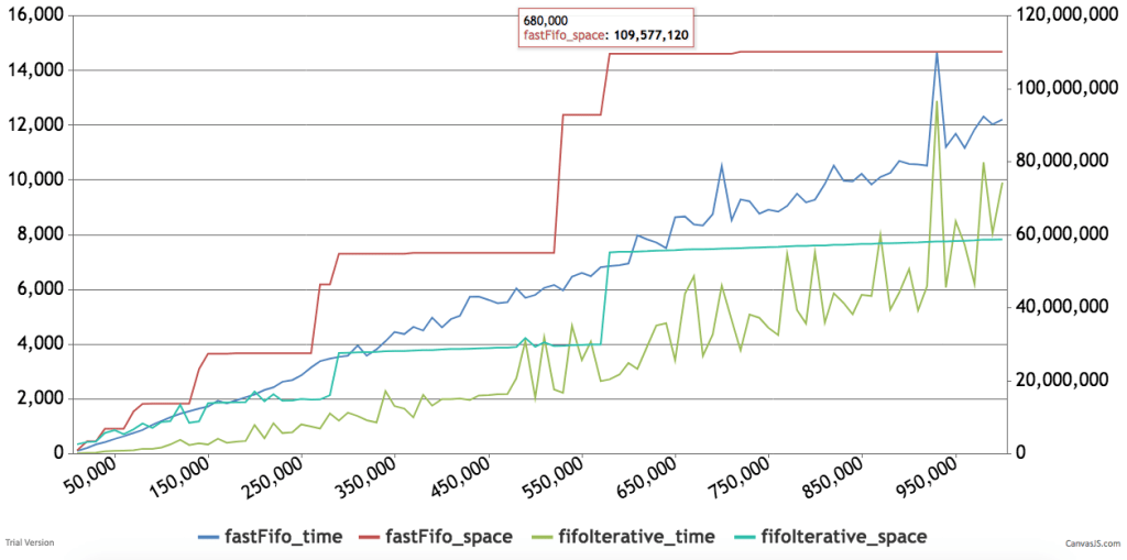
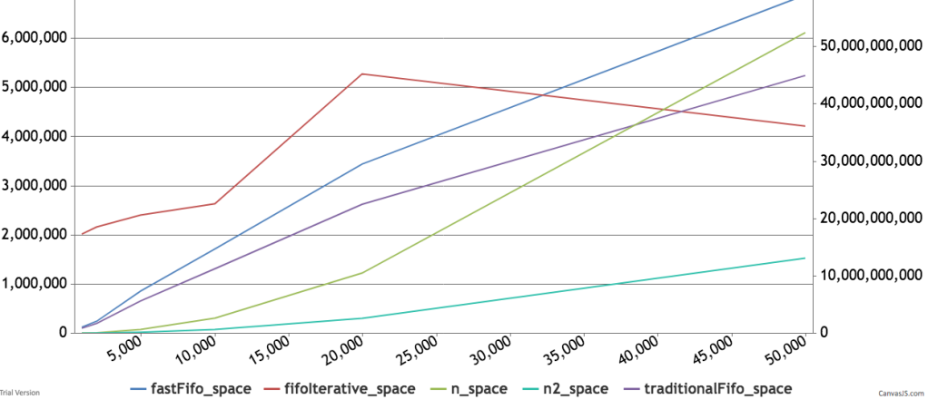
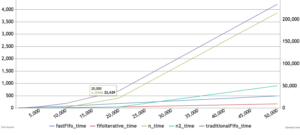
This code actually performs much faster than the iterative version and is shorter. This code essentially has no branching except where there are no more allocations on one side and exits early.
If anyone has a better way of computing fifo allocation let me know in the comments.
Below are some timings and graphs of memory usage. The code can be found here.

The Is-Ought Distinction
As a topic, the is-ought (or fact-value) distinction has been beaten to death. It is so straightforward that it is surprising to see a very intelligent person like Sam Harris completely misunderstand it.
First, let’s go over the is-ought distinction. Famously pointed out by Hume, the idea is that no set of ‘is’ statements can lead to an ‘ought’.
For example:
The person is dying.
This medicine on the counter can save her.
-> the person ought to take the medicine
This simply doesn’t follow unless you believe the person ‘ought’ to live.
Now, to show that I don’t misunderstand Sam, I’m going to steelman his position as is done in the rationalist community.
We start from a naturalist claim. Consciousness is a natural phenomenon that each of us experiences and cannot really ignore. Once we acknowledge that consciousness exists and that we are conscious beings, we must acknowledge the reality that we are programmed to avoid suffering. To illustrate this point, Sam will note that we will pull our hand off a fire. In other words, consciousness is the proximate cause of human behaviour (as opposed to the root cause, which is the big bang or whatever happened at the beginning of the universe). That cause works in predictable ways that science can study. Therefore, we can posit that the subject of a science of morality is to figure out how to achieve the types of goals that are built into the structure of consciousness in the most effective way.
The only axiom needed is that navigating away from the worst misery and suffering is a good place to start such a science.
Sam compares this field to the study of medicine, which most acknowledge is a science. The goal of medicine is to figure out what substances will cause a human to live a healthier life. So medicine generally concerns itself with efficacy of taking pain away from living things.
The only axiom underpinning medicine is that it is worthwhile to study how to keep living things, specifically human beings, healthy.
Therefore, there is nothing more special about the science of morality than the science of medicine.
Now, I will show you why Sam is wrong. What Sam seems to miss is that the ‘ought’ itself is the moral claim and is not part of the science. Simply put, medicine does not tell you that you ‘ought’ to give the dying man this pill that will save him. It only tells you that doing so ‘will’ save his life. This explains why we need the hippocratic oath in addition to the study of medicine. It also explains how Nazi doctors, who performed extremely immoral scientific studies on people, were in fact practicing a form of science. If Sam wants to study what will cause the greatest well being in conscious minds, that’s fine. There is nothing that his science will compel us to do, until we bring our values to the table.
For instance, if the person in the original syllogism who was dying was a ‘bad’ person, we arguably ought not to give her the medicine. However, the scientific fact that medicine would save her life remains. Or suppose the person is really old and wants to die, she might choose not to take the medicine. Again the scientific fact about the medicine saving her life remains. The same is true of Sam’s science of morality. It will tell you what things maximize well being without telling you what to do about them. It might be true that acting in a way that causes humanity to suffer will indeed decrease the general well being of conscious agents (indeed this seems almost tautological) and is against the desire of each agent. However, it does make a rational agent compelled to act one way or another. For instance, we can easily imagine a situation where one conscious agent wants to hurt another, because they are a psychopathic serial killer. We can imagine putting the psychopathic serial killer on drugs that will cause them to stop wanting to kill the victim. This will add to the well being of the victim and, if the drugs are really good, they might also add to the well being of the killer. However, during that intervention, forcing the drugs down the throat of the killer, will certainly add to the suffering of the killer, who wants nothing more than to strangle his victim. I am sure what the moral answer should be, but the moral science will permit me no such claims. It will only be able to measure all of the well being of all the agents and tell me how all the agents respond to different treatments.
Sam might be right, that we generally understand that the goal of medicine is helping people lead healthier lives. However, that doesn’t acknowledge where the science is a science and where it is just the overwhelming social consensus of what to do with the knowledge. He can even claim that such a distinction is not useful in medicine. although the entire field of bioethics would seem to discredit such a claim. It is also true, that any study of morality must rely on a solid foundation of facts. Those facts might belong to the field of science of morality, which will tell you the consequences of actions on conscious beings. You cannot make an informed moral decision without the facts. So the facts are a necessary, but insufficient condition for moral claims.
If Sam were right, then a science of Sadism would compel me to be a sadist. Yet, we might want to study what causes suffering and how to cause the greatest amount. This field might spawn other useful subfields such as dentistry. The choice of the field of study is in itself a value judgement, in so far as it prioritizes time across an infinite array of fields and focuses on some particular domain. For example, we can agree that the government should sponsor basic research in astronomy, but not astrology. People can disagree with that statement in many ways, but none of those claims and statements are about facts. The facts remain, that astrology studies occult things and astronomy studies the cosmos. Choosing between these disciplines is a valid choice and a sufficiently functional society can choose to allocate its resources into either field.
There is a separate argument to have with Sam’s choice of axiom. We can imagine a drug that will give everyone the conscious feeling of well being, and yet it might be immoral to force everyone to take it.
I know that Sam is very smart and so I have tried as hard as possible to defend his position in a strong way. If anyone can help me make his case stronger, that is welcome.
It’s Flooding on all sides!
This post is inspired by a happy coincidence, I was doing p2 of day 14 of advent of code for 2017 and I had never formerly encountered the flood fill algorithm. This confluence of events inspired me to come up with a new way to solve this classic problem.
You are given a boolean matrix and told that points are neighbors if they are either next to each other horizontally or vertically, but not diagonally. If point (a) and point (b) are neighbors and point (c) is a neighbor of point (b) then (a),(b) and (c) are in the same neighborhood. A point with no neighbors is a neighborhood of 1. You are asked how many such neighborhoods exist.
Shamelessly borrowing the picture from adventofcode:
11.2.3..-->
.1.2.3.4
....5.6.
7.8.55.9
.88.5...
88..5...
.8...8..
8888888.-->
|      |
V      V
You can see that this piece of the matrix, has 9 neighborhoods. Points that are off in the boolean matrix are simply ignored.
This problem is a classic because it is apparently how that bucket fill tool works in every paint program. Essentially you keep filling all the pixels that are neighbors until you are done.
Now the classical way to solve this problem is flood fill. Essentially the problem is broken into two pieces:
- An outer loop that visits every point
- An inner loop that looks for neighbors using breadth first search or depth first search
Here I will annotate the Q code that achieves this result.
ff:{[m] /this is flood fill function
	/ returns a table with all the distinct neighborhoods
	/m is a matrix
	[m]
	/c is the number of rows
	/columns this matrix has, we assume it's square
	c:count m;
	/we flatten m; m is now a list of length c*c
	m:raze m;
	/we create t, a table that is empty
          /and has columns id, and n
	 /id will be the id of the neighborhood
	 /n will be a list of neighbors in that hood
	t:([id:()]n:());
	/gni is a helper function that get neighbor indexes
	/gni will accept the index as an offset
	/ from the flattened matrix
	/and will return coordinates as flat offsets.
	/internally it needs to represent
             /the coordinates as a pair,
	/ we use standard div and mod to represent the pair
	gni: { [x;y]
	  /x is the size of the matrix it will be fixed to c
	  /y is the point
	  /s whose neighbors we want to find
	  /ny are the new col coordinates
	      / found by dividing the point by c
	      / we add the offsets
	      / but makes sure we are within boundaries of matrix
	      / min 0  and max c-1

    ny:0|(x-1)&0 -1 1 0+/:y div x;

		  /repeat this process to calculate row coordinates

    nx:0|(x-1)&-1 0 0 1+/:y mod x;

      /get back original flattened index
       /by multiplying ny by c and adding nx
      /flatten list and only return distinct points
	 distinct raze nx+x*ny
	 /project function onto c, since it will be constant
	 / for the duration of the parent function
	      }[c];

   /f is our breadth first search function
   /we start by adding i, which is our first point,
   /we then find all the gni of i,
   /we remove any gni[i] that are already present in i
   /and intersect the new points that are on (=1)
   /by intersecting with j
   /we project this function on gni,
   / which is called gni inside as well.
   /we also project on the points that are on
   /(are equal to 1) aka (where m)
   / and which are named j inside the function)
	 f:{[gni;i;j](),i,j inter gni[i] except i}[gni;;where m];
   /repeating f over and over will yield
   /  all the neighbors of a point that are on (=1)

   /now we get to the outer loop,
    /which will check
    /if we have seen the current point  (p)
   /if we have seen it, we ignore it,
    /and return our current table (t)
   /otherwise, we call f on that point and return
    /the point and all of it's neighbors
   /this will end up with our new table t,
   /we only call this function on the points
   	/that are turned on,
   /which means we can skip checking if the point is on
  /we will repeat this for all the points equal to 1
	t:{[f;m;t;p]$[not p in exec n from t;
						t upsert (p;f over p);
						t]}[f;n]/[t;where m];
  }
The entire code without comments looks like this, and is pretty short.
ff:{[m]
	c:count m;m:raze m; t:([id:()]n:());
	gni:{distinct raze (0|(x-1)&-1 0 0 1+/:y mod x)+x* 0|(x-1)&0 -1 1 0+/:y div x}[c];
	f:{[gni;i;j](),i,k where j k:gni[i] except i}[gni;;m];
	t:{[f;m;t;p]$[not p in raze exec n from t;t upsert (p;f over p);t]}[f;n]/[t;where m]
	}
With that out of the way, I now want to explain an alternate way of achieving something essentially identical.
A common technique in math and engineering fields is if you can’t solve a problem, find a similar problem that is easier that you can solve and solve that first.
So I pretended that all I needed to do was to find runs, which is a set of consecutive 1s in a row. I figured if I do this for all the rows and all the columns, I’ll have a starter set of neighborhoods and I can figure how to merge them later.
Finding a run is really simple:
- set the neighborhood id to 0
- start at the beginning of first row
- look at each element,
- if you see a 1 add element to the list that corresponds to your current neighborhood id
- if you see a zero increment the neighborhood id
- if next row, go to the next row, increment neighborhood id, otherwise go to step 8
- go to step 3
- remove neighborhood ids with no elements in them.
In q, you can take a bit of a shortcut by asking each row, for the indexes with a 1 in them. So for example:
q)where 1 0 1 1 0
0 2 3
q) deltas where 1 0 1 1 0
0 2 1
One thing we notice is that consecutive differences of 1 represent runs and those with any other number represent cut points, and if we cut at those points, we would get (,0; 2 3) which is a list that contains two lists, each inner list is a run in that row. We can repeat this for the columns and create all the runs that exist row wise or column wise.
Now we just need some logic to merge these runs. Here is an annotated version of the code that implements this method of finding all the neighborhoods.
rr:{[m] /This will return all the points in the matrix that are on and their assigned neighborhood id
	/m is the square matrix
	c:count m; /c is the length of a side of the matrix
	m:raze m; /m is now the flattened list that corresponds to the matrix
	/runs is a function that will return a list of lists,
	/each inner list corresponds to points that are adjacent
	/Though the mechanism to calculate adjacency is in terms of y
	/It will return the Xs that correspond to those Ys.
	/eg if we have a row 0 1 1 0 1 0 1 1, and the points are labeled `a`b`c`d`e`f`g`h
	/runs[0 1 1 0 1 0 1 1;`a`b`c`d`e`f`g`h] => (`b`c;,`e;`g`h)
	runs:{(where 1<>-2-': y) _  x};
	/now we want to apply runs to every row and column
	/n will be our initial list of neighborhoods,
	/ each neighborhood is a list that will contain adjacent elements either by row or by column
	/ elements are given a unique id
	/i will be our unique id , it is the index of the point that is turned on (=1)
	i:where m;
	/j groups all 'i's that are in the same row, by using integer division
	/so j is a dictionary whose keys are the row index and whose values are the 'i's
	/we need to do this grouping to ensure that only points in the same row are considered adjacent
	/ otherwise we might believe that a diagonal matrix has runs (because we only see the column indexes)
	j:i group i div c;
	/since runs returns x, but uses 'y's to do the splitting, we provide j mod c as y
	/j mod c corresponds to the column location of each i
	/we then  apply runs on (')each j and j mod c.
	/finally we flatten the result with a raze so that we just a have the list of row neighborhoods
	n:raze runs'[j;j mod c];
	/now we will repeat with the columns
	/we want to permute the list i so that the elements appear in column order
	/we want to preserve the labels we have in i
	/so we generate a list that is the length of m (c*c),
	/we reshape (#) to be a square matrix, and transpose it along the diagonal (flip)
	/we flatten(raze) it back out and intersect it with i,
	/this preserves the column order we achieved from doing the flip,
	/but only keeps the elements that are in i
	/k are the elements of i permuted along columns
	/eg if we have a matrix
	//           0 0 1
  	//           1 0 0
  	//           0 1 0
  	// i would be 2 3 7
  	// and k would be 3 7 2
	k:(raze flip (c;c)#til c*c) inter i);
    /now we will create the j  again which is our grouping
    /but this time according to the column index so we will group by the integer remainder (mod)
    /this will separate our indexes into columns
    j:k group (k mod c);
    /then we will apply our runs function on each column
    / we use the div to get the row index of each element,
    / so that runs can tell if two points are vertically adjacent
    / we flatten the result and append it to n
    n,:raze runs'[j;j div c];
    / at this point we have a list of all possible neighborhoods, but there are overlaps
    / so we create a table t, which will assign an id for each neighborhood contender
    / ungroup flattens the table so that every element belongs to a neighborhood id
    // here is a sample of what the table looks like before and after ungroup
    / before ungroup:
	/				n         id
	/				------------
	/				0 1       0
	/				,3        1
	/				,5        2
	/				8 9 10 11 3
	/after ungroup
	/				id n
	/				-----
	/				0  0
	/				0  1
	/				1  3
	/				2  5
	/				3  8
	/				3  9
	/				3  10
	/				3  11
    t:ungroup `id xkey update id:i from ([]n);
    / f is our merging function.
    / It will merge neighborhoods together,
    / by giving them the same id if there are points in common.
    / First we will update/create a column p which is the minimum id for a given element (n)
    / Then we will update all of the ids the with minimum p and rename that the new id
    / If two neighborhoods share a point in common, that point has two neighborhood id's
    / we will assign it primary id (p) which is the min of those two ids
    / we then group by id and assign the id to be the min of the primary ids (p)
    f:{[t]update id:min p by id from update p:min id by n from t};
    /On each iteration of this function we will merge some neighborhoods,
    / we repeat until we can't merge anymore
	f over t}
The uncommented code is much shorter and looks like this:
rr2:{[m]
    c:count m;m:raze m; runs:{(where 1<>-2-': y) _  x};
    n:raze runs'[j;(j:i group (i:where m) div c) mod c];
    n,:raze runs'[j;(j:k group (k:(raze flip (c;c)#til c*c) inter i) mod c) div c];
    t:ungroup `id xkey update id:i from ([]n);
    f:{[t]update id:min p by id from update p:min id by n from t};
    f over t}
At this point we are done and we have solved the puzzle in two slightly different ways. Looking at the performance of both methods, reveals that they are both O(n) essentially linear in the number of elements. However, the row method is actually faster, because everything is done as nice straight rows, so there is not much jumping around, in other words it is more cpu cache friendly. On my late 2011 Mac: for a 128 by 128 matrix
\t rr m
176 milliseconds
\t ff m
261 milliseconds
So it is about 66% faster
As a bonus, my father suggested that I expand this code into n dimensions. This is rather easy to do and I include the code here without too many comments. The trick is taking advantage of KDB’s vs (vector from scalar) function that can rewrite an integer as a number in another base:
so for example 3 vs 8 => (2;2) which are the coordinates of the point 8 in a 3 by 3 matrix. The point 25 is 2 2 1, in other words it’s in the last layer of a 3 dimensional cube of size 3, last column and first row.
This means we can easily go back and forth between integer representation of the matrix and coordinate representation. Everything else is pretty much the same.
ffN:{[m]
    c:count m;r:1; while[(count m:raze m)<>count[m];r+:1]; t:([id:()]n:());
    gniN:{[r;c;n]a:neg[a],a:a where 1=sum each a:(cross/)(r;2)#01b;
        distinct raze -1 _ flip c sv flip (c-1)&0|a +\: c vs n,-1+prd r#c}[r;c];
    f:{[gni;i;j](),i,j inter gni[i] except i}[gniN;;where m];
    ps:where m;
    while[count ps;t:t upsert (first ps;k:f over first ps); ps:ps except k];
    /functional version is slower
    /t:{[f;t;j]q+::1;$[not j in raze exec n from t;t upsert (j;f over j);t]}[f]/[t;where m]
    t}

rrN:{[m]
    c:count m;r:1; while[(count m:raze m)<>count[m];r+:1]; runs:{(where 1<>-2-': y) _ x};
    j:(c sv (til r) rotate\: c vs til prd r#c) inter\: where m;
    g:til[r] except/: d:reverse til r;
    n:raze raze each runs''[j@'k;@'[v;d]@'k:('[group;flip]) each @'[v:flip c vs j;g]];
    t:ungroup `id xkey update id:i from ([]n);
    f:{[t]update id:min p by id from update p:min id by n from t};
    f over t}
